INTRODUCTION

As is typical across all energy generation systems, accurate characterization of system losses is essential for setting generation expectations. For instance, it is long understood that turbine performance, turbine unavailability, wind-reducing wakes from obstacles and other turbines, environmental impacts, curtailment, and other causes can lead to considerable energy loss in a wind project. Utility-scale wind energy researchers and industry players have used the wealth of turbine operations information available to quantify and categorize production loss. For example, Staffell and Green [1] determined that wind turbines in onshore utility-scale projects in the United Kingdom lose 1.6% of their generation output per year due to age-related performance decline. Ribeiro and Beckford [2] analyzed wind farms in Scandinavia and found that production loss due to icing could exceed 50% during winter months and 10% over the course of a year. El-Asha et al. [3] performed a diagnostic study of a wind farm in the United States and established typical wake losses of 2%–4% that could reach 60%–80% for some wind turbines in the farm during specific wind direction conditions. Wind farms analysts continue to use observation-based loss research to improve energy production expectations for existing and future projects.

Distributed wind projects are connected at the distribution source of an electricity system or in off-grid applications. These projects, which can utilize one or more turbines with capacities ranging from less than 1-kilowatt to multi-megawatt, serve onsite or local energy needs. In contrast with the utility-scale wind energy industry, the distributed wind community suffers from a dearth of publicly available information on project loss. For example, the National Laboratory of the Rockies’s (NLR) Cost of Wind Energy Review [4] and Distributed Wind Energy Futures Study [5] report estimates of the levelized cost of energy and technical potential, respectively, for distributed wind projects in the United States. Both reports incorporate a loss factor of 16.5% to represent energy loss due to blade soiling, turbine controls, and grid and turbine availability (Table 1). The source of the 16.5% loss factor is attributed by Stehly et al. [4] as informed by NLR’s Competitiveness Improvement Project [6], which provides financial and technical support to manufacturers of small wind turbines, with no elaboration on the quantity or models of the turbines involved in the quantification, nor the temporal coverage, weather conditions, or loss categories involved.

Contemporary tools that serve distributed wind customers present a range of loss categories and default loss factor values for converting gross wind energy estimates to net wind energy estimates (Table 1) but lack accompanying information to explain why the default values are selected. To support distributed wind energy customers, the Distributed Wind Energy Association (DWEA) developed the wind feasibility tool AgWind which utilizes a 10% turbulence factor to adjust gross energy estimates to net [7]. The NLR System Advisor Model (SAM) provides techno-economic analysis of a range of energy technologies, including utility-scale and distributed wind energy. For both utility-scale and distributed wind energy, SAM considers a comprehensive suite of loss categories, including wake, availability, electrical, turbine performance, environmental, and curtailment losses, which sum to a total default loss assumption of 18% [8]. Global Wind Atlas is a widely used application created by the Technical University of Denmark (DTU) and the World Bank Group to assist policymakers, planners, and investors in identifying locations for wind power generation. Global Wind Atlas has a default loss assumption of 10% to cover wake and availability loss [9]. DTU is also the developer of MyWindTurbine, a tool for determining the feasibility of single-installation small and midsize wind turbines [10] with a default loss assumption value of 7% [11] to cover technical loss but not wake loss [12].

TABLE 1

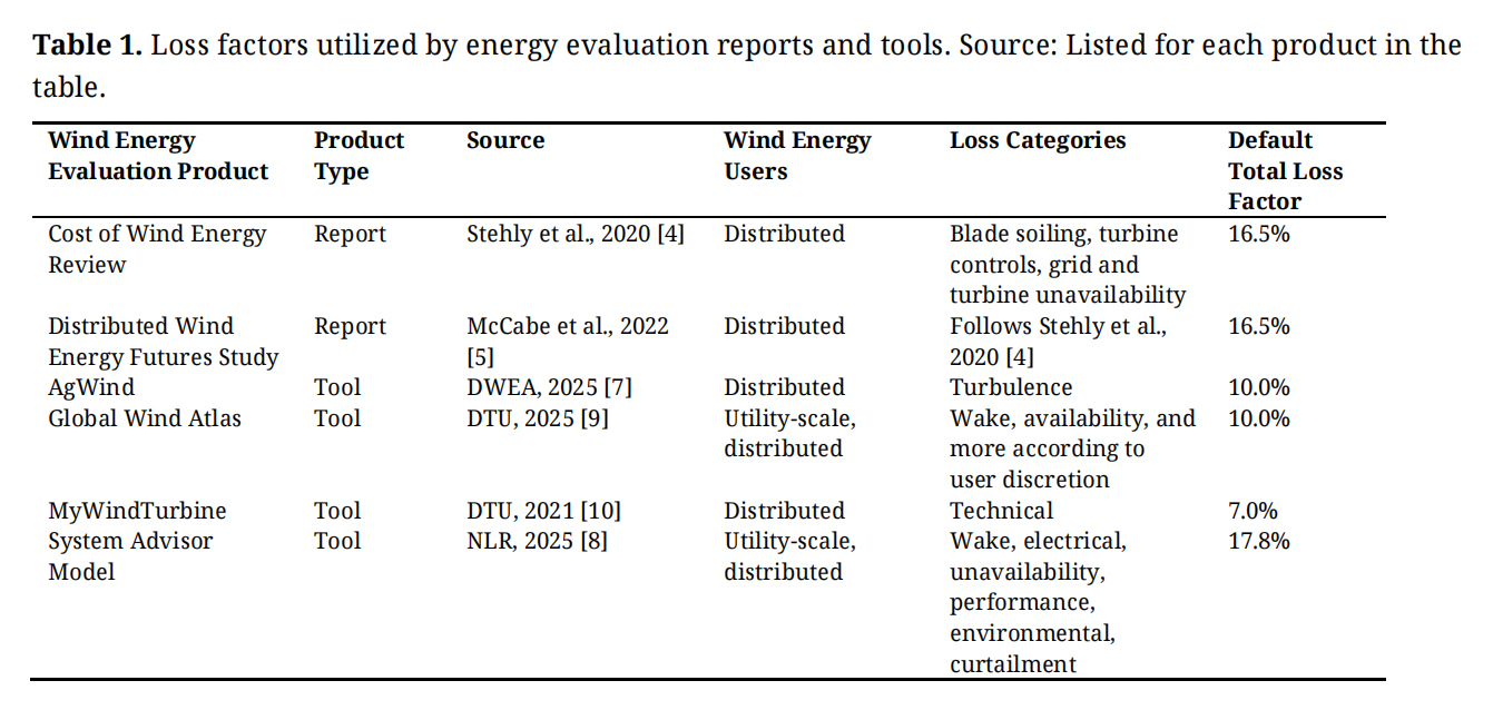Table 1. Loss factors utilized by energy evaluation reports and tools. Source: Listed for each product in the table.

We hypothesize that loss assumptions for distributed wind tools will improve if operational observations from real world projects are accounted for. This work utilizes generation observations from distributed wind projects consisting of small wind turbines (nominal capacity ≤ 100 kW) installed across the United States with the goal of establishing more accurate default loss factors for distributed wind energy estimation tools, in particular, NLR’s WindWatts [13]. The distributed wind projects fall into a typical design and ownership scenario observed in Pacific Northwest National Laboratory’s (PNNL) Distributed Wind Project Database [14]: small, locally owned, geographically scattered, single installation wind turbines. The Data and Methods Section shares the background on the distributed wind turbine observations, models and datasets, and methodology used to establish loss factors for distributed wind projects. Additionally, the Data and Methods Section includes a deep dive into the frequency of occurrence of different types of energy loss experienced by the turbines. Next, the Results and Discussion section establishes loss factors for small distributed wind projects and explores trends in loss according to geographic region and proximity to turbine service providers. Finally, the Conclusions section summarizes the findings and speaks to the impacts for distributed wind customers.

DATA AND METHODS

The process to determine energy loss for distributed wind projects follows a measure-correlate-predict protocol, beginning with filtering each turbine dataset to exclude abnormal, underperforming, or missing time periods. The remaining “normal” data are subsequently trained with reference atmospheric model data using a machine learning technique to establish a relationship between the observed and simulated datasets. This relationship is then applied to the reference atmospheric model data during times when the turbine measurements are missing or did not pass the filtration protocol to predict what the turbine production should have been during periods of abnormal, underperforming, or offline events. The following sections provide deeper information on the wind turbine observations, the reference atmospheric model data, the filtration procedure, and the machine learning methodology.

Wind project generation timeseries from distributed wind commercial entities are graciously shared with our team in a joint public-private effort to improve wind energy estimates. The wind generation data collection includes power output and nacelle wind speeds that have been corrected to estimate the free stream wind according to each commercial entity’s unique nacelle transfer function. The data from the turbines, which are shared with the authors under public-private partnership agreements to improve wind energy estimates in the WindWatts tool [13], support distributed wind loss evaluation for a typical distributed wind project design and ownership scenario involving a single small wind turbine.

The small wind project dataset consists of operational data from 72 projects using single-installation small wind turbines (capacities ≤ 100 kW). The small wind projects are owned by the specific customer receiving the energy produced or by local utilities and are installed across the continental United States, Hawaii, and Alaska. Our study collection focuses on small wind projects installed in the Midwest (33 projects), Southern Plains (9 projects), and Northeast (30 projects) regions of the United States due to the higher sample sizes found in these areas (Figure 1). The interconnection types of the projects are either behind-the-meter or via grid-connected microgrids, load-serving distribution lines, or remote net-metering. Turbine hub heights for the projects are less than 50 m.

FIGURE 1

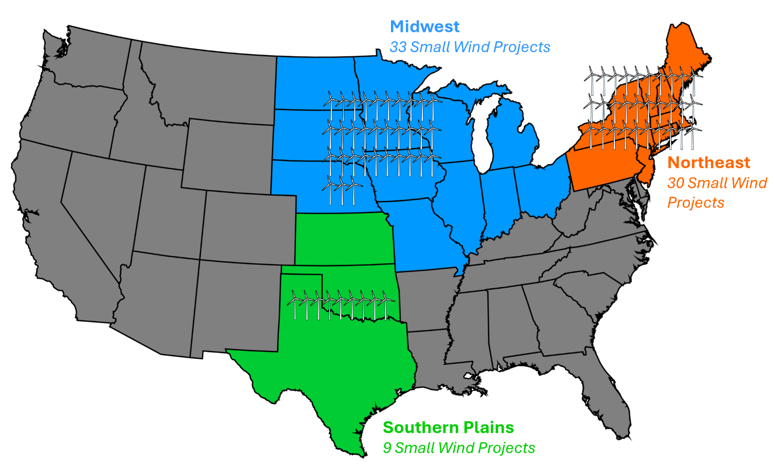Figure 1. Map of United States regions and sample sizes of small distributed wind projects in this study. Source: Own research.

The wind power generation datasets output at a 10-minute output frequency. We subsample the generation timeseries to keep only reports at the top of the hour to temporally align with the 1-hour resolutions of the reference atmospheric model datasets used during the correlate and predict phases of the loss analysis. Additionally, to align with the coverage periods of the atmospheric reference datasets, we limit our analysis to the years 2015 to 2023. The turbines were installed between 2008 and 2016, resulting in temporal duration ranges for this analysis of 2 to 8 years with a median of 8 years.

The success of every measure-correlate-predict application depends on the quality of the observations gathered in the measure phase; therefore, we apply the following filtering procedure to establish high quality datasets for training in the correlate phase. To make the turbine observation filtration generalizable across multiple turbine models, which have unique status and performance reporting standards, the following process requires only the turbine power output, the nacelle wind speed, and the manufacturer’s power curve. We acknowledge that this approach has both advantages, including simplicity and application to multiple turbine models, and limitations, when considering the lack of service logs and weather information beyond wind speed that could result in even higher quality datasets.

We use density-based spatial clustering, specifically Matlab’s dbscan [15], to organize the observed wind turbine power curve (nacelle wind speed versus turbine power output) into normal and abnormal performance clusters (Figure 2). The normal performance clusters are used to build relationships with the atmospheric models. The abnormal performance clusters are used to establish loss by comparing the actual turbine power production with what should have been produced based on the relationship built during times of normal performance.

For each small wind turbine, we iterate over 1-kW segments of observed turbine power data. For each 1-kW segment, we assess whether that segment falls along the steep portion of the power curve, when power increases significantly with wind speed, or the flatter top portion of the power curve near the turbine’s nominal capacity. If the segment being filtered occurs in the steep portion of the power curve, we apply an epsilon neighborhood search radius of 1 m s⁻¹ that must contain at least 50% of the points within the segment. If the segment occurs at the top of the power curve, we use an epsilon neighborhood search radius of 10 m s⁻¹ that must contain at least 90% of the points within the segment.

The density-based clustering approach works to cleanly filter many of the turbines in the shared collections into normal and abnormal categories, excepting several small wind turbines that experienced significant curtailment. To ensure appropriate filtering, we add a threshold prior to the clustering based on the manufacturer’s power curve. In this approach, we adjust the manufacturer’s power curve by adding 10% to the wind speeds along the steep portion of the curve while retaining the same power values. For each instance in a turbine’s observed timeseries, we linearly interpolate the nacelle wind speed with the adjusted manufacturer's power curve to determine the associated power threshold. For the flat top of the power curve, the power threshold is set to the manufacturer’s power curve power minus 10% of the nominal capacity. If the observed turbine power meets or exceeds the threshold, the point moves onto the clustering phase. If the observed turbine power is less than the threshold, it is flagged as abnormal performance. The adjusted manufacturer’s power curve threshold approach is applied to all turbines in the small wind collection prior to the clustering evaluation.

The review of applications and modelling techniques of wind turbine power curves for wind farms performed by Bilendo et al. [16] identifies five main categories of the most common power curve anomalies corresponding to abnormal performance: (1) lower stacked data (power at or near zero for wind speeds greater than cut-in and less than cut-out), (2) downrating or curtailment, (3) wind speed under-reading (persistence of higher than anticipated power generation for lower wind speeds), (4) dispersive (spread) data, and (5) icing/debris build-up on blades. Across the distributed wind observations in this analysis, all five categories can be identified, with the first four represented in the example power curve in Figure 2.

FIGURE 2

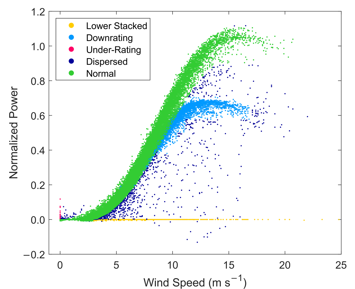Figure 2. Example of the filtering process applied to an actual small distributed wind power curve used in this analysis. Power is normalized using the turbine’s nominal capacity. Source: Own research.

Figure 3 shares the estimated frequency of occurrence per project of the five main categories of power curve anomalies identified by Bilendo et al. [16], along with the frequency of normal performance and missing power reports. It is important to note that Bilendo et al. [16] do not provide specific numeric guidelines for parsing power curve data into the five main categories; therefore, the values presented in Figure 3 are estimates based on the visual signatures of power curve anomalies and should be treated as such. In addition to the power curve anomalies, we also consider turbine unavailability when data is not being reported, which could result from planned or unplanned downtime or communication issues. As all the distributed wind projects in this study involve single turbine installations, wake impacts to energy production are not considered.

Across the 72 projects, the observed generation data indicates normal operational performance for the majority of the analysis periods for small distributed wind projects, with a median frequency of normal operations of 73%. The good quality data are kept to supply the target data for the training phase to develop models for simulating energy generation during periods of anomalous performance or lack of reports. Unavailability is the next most frequent impact to performance data, affecting a median of 15% of the study periods for the small wind turbines. Of the power curve anomalies, occurrences of lower stacked data are noted during 4% of the small distributed wind timeseries, while dispersed data occur at a median frequency of 1%. Considering the medians across the projects, downrating, wind speed under-rating, and icing/debris events occurred less than 1% of the study periods, though some small wind projects experience downrating up to 48% of their operational timeseries (Figure 3).

FIGURE 3

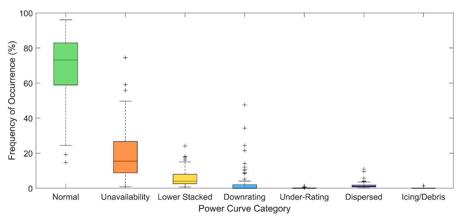Figure 3. Frequency of occurrence of power curve anomalies across 72 small distributed wind projects. For this and all box-and-whisker plots in the manuscript, the median value is indicated with the horizontal line within each box, the 25th and 75th percentiles form the box ranges, and the minimum and maximum values excluding outliers are displayed as the whiskers. Any outliers are indicated with + symbols. Source: Own research.

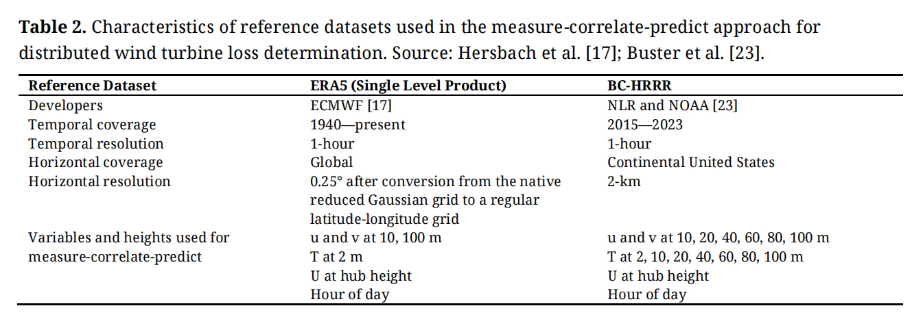
We explore two reference datasets for the correlate and predict phases of the loss factor determination study, beginning with the widely used European Centre for Medium-Range Weather Forecasts (ECMWF) Reanalysis version 5 (ERA5). ERA5 is a global reanalysis model [17] used in wind energy evaluations in a number of ways, including measure-correlate-predict assessments, due to its tendency to have high correlation accuracy with wind observations [11,18,19]. ERA5 provides atmospheric, land surface, and oceanic reanalysis data from 1940 to the present time across the globe at a horizontal resolution of 0.25° after conversion from the native reduced Gaussian grid to a regular latitude-longitude grid (Table 2, [17]). For the correlate and predict phases of determining distributed wind turbine loss, we select the u and v components of the wind at 10 m and 100 m above the ground and the temperature T at 2 m above the ground from the ERA5 single level product [20] as reference variables.

The second reference dataset we consider is less broadly validated, being more recently released, with higher horizontal and vertical spatial resolution. In a partnership with the National Oceanic and Atmospheric Administration (NOAA), NLR interpolated and bias-corrected the High-Resolution Rapid Refresh atmospheric model [21] with the WIND Toolkit (WTK) [22] to create the Bias-Corrected HRRR (BC-HRRR) [23], which is publicly available via NLR’s Wind Resource Database [24]. To develop BC-HRRR, Buster at al. [23] interpolated the HRRR data at forecast hour 2 from the model’s original grid at 3-km resolution to the WTK grid (2-km resolution) using inverse distance-weighted interpolation. The NLR team next applied quantile mapping bias correction to the HRRR data during the years 2015 to 2023 using the WTK (temporal coverage = 2007 to 2013) as a historical baseline [23]. For the correlate and predict phases of determining distributed wind turbine loss, we convert the BC-HRRR wind speeds and wind directions at 10 m and every 20 m between 20 m and 100 m above the ground to the u and v components of wind. Additionally, we select T at the same output heights as the wind components, along with 2 m above the ground, to include in the reference set of variables (Table 2).

For both ERA5 and BC-HRRR, we supplement the reference sets of variables with the hour of the day and the wind speed at each turbine’s hub height. In cases when the turbine hub height does not align with an output height for the wind variables in a dataset, we use the power law (Equation (2)) with a shear exponent calculated at each timestamp in the reference timeseries (Equation (1)) using the wind speeds U_lo and U_hi at the nearest output heights z_lo and z_hi surrounding the turbine hub height to determine the wind speed at this level (U_hub).

$\alpha = \frac{\ln \left((U_{hi}/U_{lo})\right)}{\ln \left((z_{hi}/z_{lo})\right)}$ (1)

$U_{hub} = U_{lo}{\left(\left(\frac{z}{z_{lo}}\right)\right)}^{\alpha }$ (2)

We use the nearest neighbor grid point to each turbine location to develop the reference datasets from ERA5 and BC-HRRR for the correlate and predict phases.

TABLE 2

Table 2. Characteristics of reference datasets used in the measure-correlate-predict approach for distributed wind turbine loss determination. Source: Hersbach et al. [17]; Buster et al. [23].

Once the wind power observations are filtered according to the method outlined in the Data Filtering section, we establish a training dataset of timestamps, observed generation, and reference variables from ERA5 and BC-HRRR (Table 2) for each distributed wind turbine that satisfies the following criteria:

We next develop trained regression models with ERA5 and BC-HRRR individually supplying the predictors for the wind generation observations that meet the expected performance criteria as the target. Two regression models are explored for their potential to develop representative timeseries of observed wind generation: (1) regression trees using Matlab’s fitrensemble [25] with 100 trees and (2) neural networks using Matlab’s fitrnet [26]. To test the accuracy of the combinations of these approaches and atmospheric models prior to extending any of them to simulate periods of atypical or missing generation, we withhold a randomly selected 25% of the data points from each distributed wind project’s observational timeseries as the test datasets. We designate the remaining 75% of the timeseries from each project as training datasets to predict the withheld test datasets for each project. To develop a robust sample of the performance of each combination of regression algorithm and atmospheric reference dataset, we run 30 trials of this exercise of withholding and predicting a randomly selected 25% of the filtered data for each distributed wind project.

Based on the results of the trials shown in Figure 4, we establish that neural networks in combination with BC-HRRR provides the optimal combination for predicting distributed wind generation during the redacted periods. When taking the median across the 30 trials for each site, using regression trees with ERA5 and BC-HRRR and neural networks with BC-HRRR result in the most accurate median actual versus predicted generation across the sites at 99.9% for all combinations, while neural networks in combination with BC-HRRR produces the smallest range of actual versus predicted generation (99.3–100.3%) (Figure 4a). Considering an additional error metric, the Pearson correlation coefficient is also the highest when comparing the redacted actual generation with the simulations produced using neural networks with BC-HRRR (0.75–0.90 across the 72 sites with a median of 0.86) (Figure 4b).

FIGURE 4

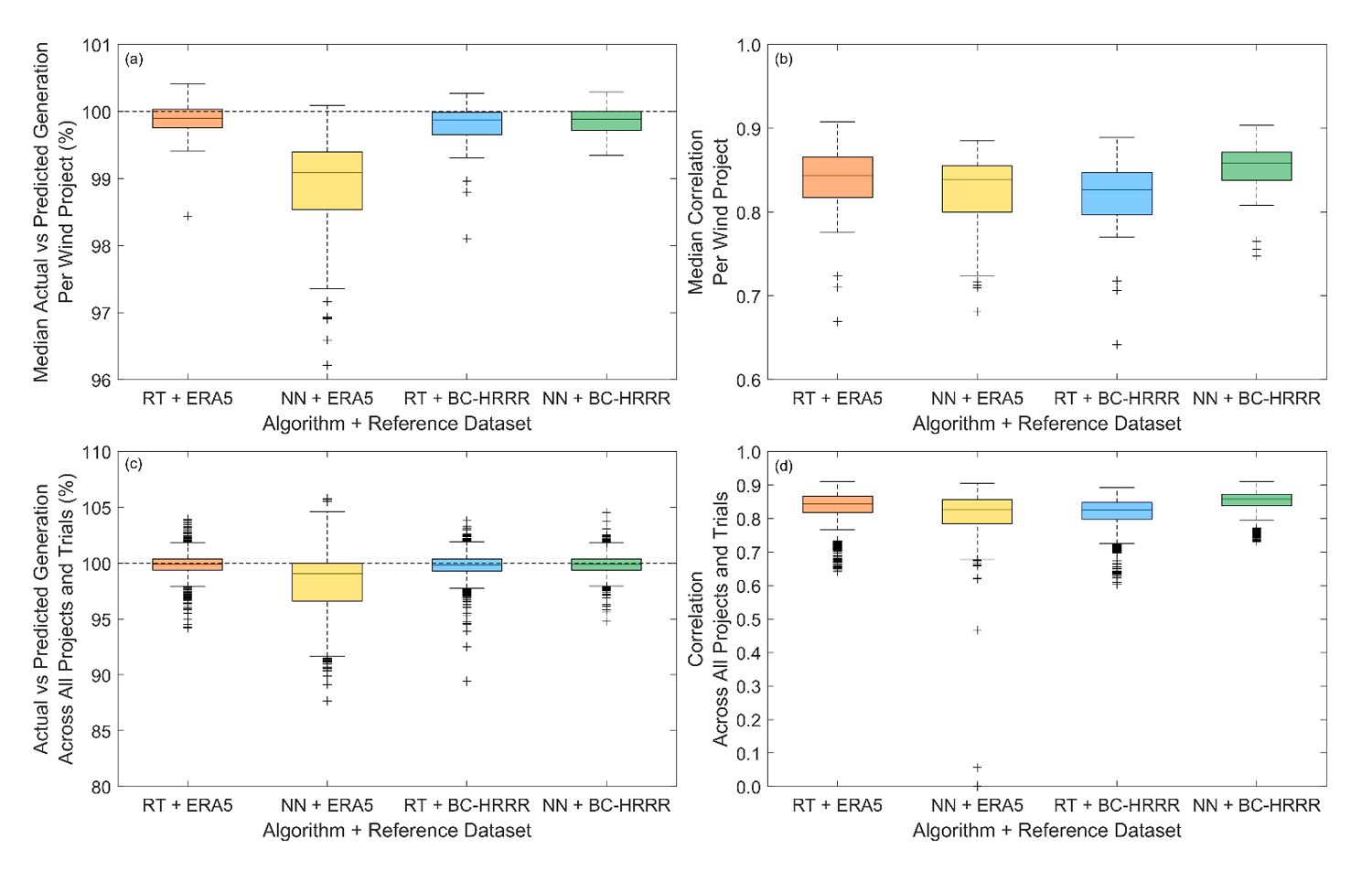Figure 4. Median per project (a,b) and full suite (c,d) of actual versus predicted generation (a,c) and Pearson correlation coefficients (b,d) between actual and predicted generation across 30 trial simulations for each of the 72 distributed wind projects using different combinations of regression-based training algorithms and atmospheric reference datasets. Source: Own research.

Interestingly, neural networks in combination with ERA5 issue the worst performance (median actual vs. predicted generation = 99.1% and range = 96.2–100.1%) despite this algorithm working more successfully with BC-HRRR (Figure 4a). We found in our trials that neural networks in combination with ERA5 exhibited challenges with learning, particularly characterized by the models being pushed toward incorrect boundaries, which we did not see for the other three combinations of algorithms and reference datasets. ERA5 is known for being well correlated with wind observations [27] but also has an established low wind speed bias [28]. We speculate that the low ERA5 wind speed bias contributes to the challenges experienced by the neural networks when trying to develop relationships with wind generation data. Based on our trials with the filtered datasets, we proceed using neural networks with BC-HRRR to build models based on the filtered datasets (again, 30 for each distributed wind project) and use them to simulate periods of atypical or unavailable turbine data.

In Figure 4c,d we include the actual versus predicted generation and correlation, respectively, across all projects and all trials to gauge the potential uncertainty for the loss determination methodology for each combination of algorithm and reference dataset if a wind analyst were to perform a single trial. Given 30 trials for each of 72 distributed wind projects, the sample size for the uncertainty calculation for each combination of algorithm and reference dataset is 2160. Across the samples, confidence is high that regression trees with ERA5 or BC-HRRR or neural networks with BC-HRRR can accurately recreate the total actual generation, with 25th and 75th percentile actual versus predicted generation ranging from 99.3% to 100.4% (Figure 4c). Including the outliers, our selection of neural networks with BC-HRRR yields the smallest range of actual versus predicted generation (94.8% to 104.5%) (Figure 4c). In terms of correlation between the actual and predicted timeseries across the samples, the 25th and 75th percentiles are similar for all four combinations of algorithm and reference dataset (0.82 and 0.87 for regression trees with ERA5, 0.78 and 0.86 for neural networks with ERA5, 0.80 and 0.85 for regression trees with BC-HRRR, and 0.84 and 0.87 for neural networks with BC-HRRR) (Figure 4d). Including the outliers, neural networks with BC-HRRR produces the smallest range of correlation possibilities and those closest to one (0.73 and 0.91) (Figure 4d).

The methodology for establishing distributed wind loss factors follows a similar protocol to the testing and validation for the expected generation observations discussed in the prior section. We develop 30 trained neural network models for each distributed wind project with BC-HRRR providing the predictors and the entire filtered generation timeseries exhibiting typical behavior as the response. The resultant neural network models are then applied to the atypical and unavailable events, with BC-HRRR as the predictor. The full estimated generation timeseries for each project is then reconstructed by combining the filtered generation timeseries exhibiting typical performance with the median of the 30 generation estimates during periods of atypical behavior or unavailable data. For each calendar year in each turbine’s generation timeseries, the loss factor is calculated according to Equation (3):

$Loss Factor=100* \left((1- \frac{Observed Energy}{Estimated Energy})\right)$ (3)

Since this analysis aims to provide typical observation-based loss factors that can be applied to distributed wind energy estimation tools and technical assistance evaluations, we exclude cases of extreme outages when calculating the loss factors. We define extreme outages as calendar years with no generation reports and the surrounding calendar years on both sides of the outage year. This approach leads to the exclusion of 39 analysis years across 11 small wind projects for the loss factor calculations. Each of the small wind projects that are impacted by data removal contains valid years that are included in the loss factor analysis. Unless otherwise specified, deep dive analyses that focus solely on turbine unavailability include all study years, including those with extreme outages, to establish trends according to turbine age and year of operation.

RESULTS AND DISCUSSION

The medians of the annual loss factors for the 72 small distributed wind projects are highly variable, ranging from 2–66% (median across all projects = 17%) (Figure 5), corresponding with the wide degree of unavailability seen across the projects (Figure 3). The interannual variability in each small wind project’s loss can also be significant depending on the degree of unavailable data, with annual loss factors spanning 91 percentage points for one project in the Northeast with loss factors ranging from 5% to 96% over an 8-year analysis period. In fact, the median per project range of annual loss factors is 44 percentage points, highlighting challenges in turbine downtime and reporting reliability for small wind projects. In the context of wind energy estimation tools, which sometimes account for the impacts of interannual variability in the wind resource, the quantification of the interannual variability of energy loss for small wind turbines points to an important estimation gap.

This investigation highlights several similarities and differences when comparing loss for single-installation small distributed wind turbines versus large, utility-scale wind farms. Excluding wake loss in multiple turbine environments, which Lee and Fields [29] identify as the largest contributor to utility-scale wind farm loss, turbine unavailability is the most significant loss category in terms of frequency of occurrence and contribution to total loss for both small distributed wind turbines and utility-scale wind farms. In terms of total loss, however, the differences between the two types of wind energy project are substantial. The review of Lee and Fields [29] reports total losses for utility-scale wind farms ranging from 10% to 23%, while this study yields a significantly broader range of total losses for single installation small distributed wind turbines, 2% to 66%.

FIGURE 5

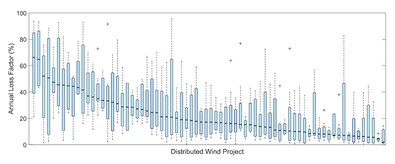Figure 5. Annual loss factors per distributed wind project. Median loss factors are highlighted with thick black lines. Source: Own research.

A wind turbine’s location can impact the degree of energy loss, and therefore the annual energy production of a project. From a regional perspective, trends in project loss can be influenced by the local environment, including frequency and severity of weather events, terrain, and proximity to wildlife populations. Separating the loss category analysis of Figure 3 by region, small distributed wind projects located in the Northeast have the greatest percentage (median = 85%) of reported and normal power curve behavior, followed by projects in the Midwest (76%) and Southern Plains (70%) (Figure 6a). Challenges related to turbine unavailability are most frequent in the Midwest, with a median of 12% of generation data in these regions being unreported during the years considered for developing loss factors. When considering the power curve anomalies, projects in the Southern Plains are the most impacted across the categories, with the sole exception of icing/debris, which only one project in the Midwest accounted for. Projects in the Southern Plains experience lower stacked anomalies around 5% of their analyzed time, compared with 2% for Midwest and Northeast projects. According to the literature review performed by Bilendo et al. [16], lower stacked events are typically caused by damage to power measuring instrumentation or communication equipment faults. Projects in the Southern Plains are the only ones to have notable frequencies of turbine derating (1%). The median frequencies of occurrence of wind speed under-rating are less than 1% across all three regions. Dispersed data accounts for 2% of the analyzed timeseries for projects in the Southern Plains, compared with 1% for those located in the Midwest and Northeast.

Driven mainly by turbine unavailability and a combination of unavailability and power curve anomalies, respectively, customers in the Midwest and Southern Plains are able to reasonably expect project loss factors of 19% and 18% compared to what their project would have documented under ideal reporting and operating conditions. Customers in the Northeast can expect slightly smaller loss factors around 16% (Figure 6b).

FIGURE 6

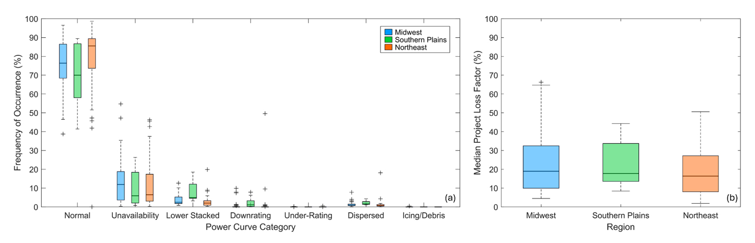Figure 6. (a) Median annual power curve anomaly frequency according to region of small wind project. (b) Median annual project loss factors for small distributed wind projects according to region. Source: Own research.

A challenge for small, locally owned, and geographically scattered distributed wind projects is access to wind turbine service providers, of which relatively few are active in the United States. The amount of time a broken or underperforming turbine is offline or not generating as expected is correlated to the time it takes for a service provider to access the turbine. Additionally, some service providers have distance ranges that they operate within, making it challenging for turbine owners to identify and access maintenance for their area. NLR maintains a list of distributed wind installers [30] to support current and future customers of distributed wind. Many of these installers also provide scheduled and unscheduled maintenance and end-of-life decommissioning for a variety of wind turbine models and sometimes other energy technologies, like solar and battery storage.

For the small wind projects, we establish the minimum distance between each distributed wind project in our analysis collection and the nearest service provider from NLR’s distributed wind installers list. The resultant distances between distributed wind projects and the nearest service provider range from 5 to 1032 km with a median of 223 km. We examine the range of annual loss factors for each distributed wind project, recalling from Figure 5 that the annual variability is quite large, according to distance to the nearest service provider (Figure 7) to test the hypothesis that proximity to turbine service is an important factor in project performance consistency. The sample of turbines in each distance bin in Figure 7 is roughly comparable, ranging from 11 to 17 turbines. While the median and maximum ranges of annual loss factors are noted to be smallest when the nearest service provider is within 200 km of the turbine, it is difficult to establish a confident relationship when no linear trend between annual loss factor range and service provider proximity is present (Figure 7).

FIGURE 7

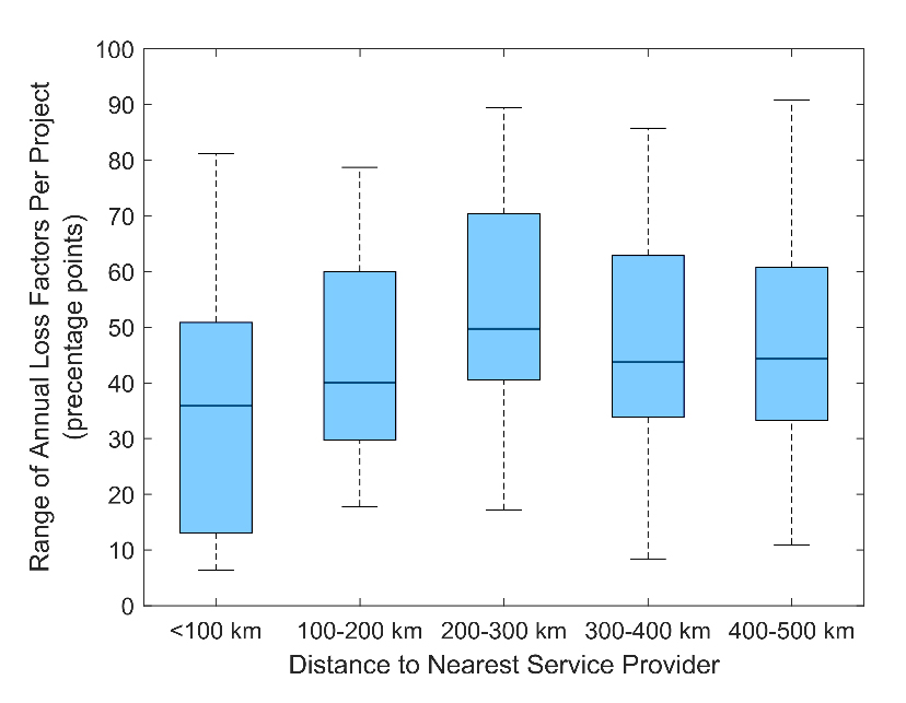Figure 7. Range of annual loss factors for distributed wind projects according to distance from nearest service provider. For each project, the range of annual loss factor is the difference between the highest and lowest annual loss factor. Source: Own research.

To explore a similar investigation to Staffell and Green [1], who determined that wind turbines in onshore utility-scale projects in the United Kingdom lose 16% of their generation output per decade due to age-related performance decline, on a small wind project scale, we examine trends in project loss according to turbine age in Figure 8. Since Staffell and Green [1] speculated that the age-related decline in utility-scale generation is due to unavailability and wear and this study identifies turbine unavailability as the biggest contributor to small distributed wind project loss (Figure 3), we focus on turbine unavailability during the first decade of a small wind turbine’s life cycle. This look back in time requires us to expand our analysis to include years outside the range covered by BC-HRRR and years of extreme outages to maintain a consistent year-to-year analysis. Of the 72 small wind turbines in the collection, roughly half (33) have consistent reporting for each year of their first decade online.

Contrary to the evaluation of Staffell and Green [1], we find no trend in small wind turbine unavailability related to turbine age during the first decade that the projects were online (Figure 8). In fact, the age at which the greatest number of turbines (8 of the 33 projects) experiences their smallest percentage of unavailability is 10 years. The age at which the greatest number of turbines (again, 8 of the 33 projects) experiences their largest percentage of unavailability is 8 years.

FIGURE 8

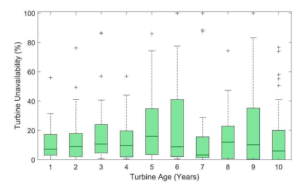Figure 8. Unavailability according to turbine age for a subset of 33 small wind projects. Source: Own research.

Without further documentation, it is difficult to attribute the variations in distributed wind project loss to specific events, characteristics, or trends. For example, Figure 9 explores turbine unavailability for a consistent subset of projects (27 in the Midwest, 8 in the Southern Plains, and 24 in the Northeast), much like the analysis in Figure 8 but for year of turbine generation. We note a significant increase in unavailability for turbines in the Northeast during the year 2021 (median frequency = 23%) which is tempting to attribute to a number of extreme weather events that occurred, including Winter Storm Orlena [31] and Hurricane Ida [32]. However, without service records or media reports, the latter of which are commonly available for incidents at large utility-scale wind farms, it is not possible to localize the impacts of the storms to the small distributed wind projects in our study collection. The observations utilized in this work provide immense value for quantifying small wind project loss factors and their year-to-year uncertainty, along with the frequency of occurrence different power curve anomalies. However, small wind energy observations tend to lack the documentation to support a full explanation as to why such interannual variations and anomalies are occurring, urging further public-private partnerships, expanded reporting guidance, and a deeper understanding of the roles and responsibilities for small, customer-owned wind projects when it comes to performance-based monitoring and response.

FIGURE 9

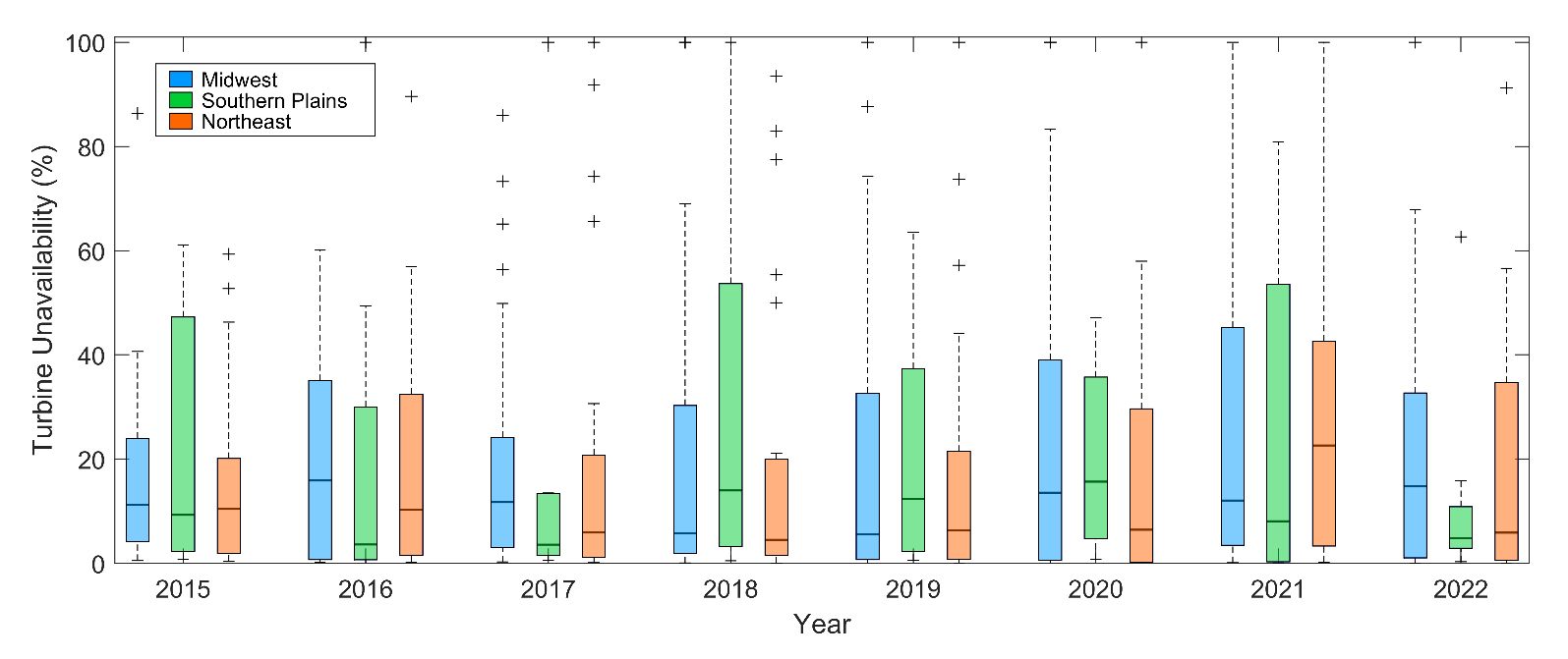Figure 9. Turbine unavailability per region and year for 59 small wind projects in the United States. Source: Own research.

CONCLUSIONS

To further underscore the necessity of accurately characterizing loss in distributed wind energy estimates, we perform a brief complementary economic analysis using the WINDVALT tool. WINDVALT is a publicly accessible webtool developed by PNNL to quickly compare costs and benefits of distributed wind systems based on user inputs [33]. In this example, a representative behind-the-meter wind turbine with a 40-m hub height sited at a windy location in Iowa is selected as an economic case study using NLR’s 100-kW reference power curve [34]. Using the above wind project characteristics with identical financial inputs, we vary the total loss assumption within WINDVALT between 7% and 18%, representing the lower and upper default loss assumptions found in distributed wind reports and tools (Table 1). The results of the case study indicate that changes in turbine loss can substantially influence project economics. Varying the WINDVALT total loss assumption from 7% to 18% for our hypothetical turbine in Iowa leads to an approximately 60% reduction in the estimated net present value of the project, demonstrating the sensitivity of small distributed wind economics to assumed loss factors.

Given the importance of accurately representing loss in distributed wind energy estimates for projects using small wind turbines, we establish observation-informed loss factors for converting gross energy estimates to net energy estimates for wind resource assessment tools and technical assistance. This research fills an important gap for wind energy estimation, as the typical characteristics of a small distributed wind project (shorter hub heights, smaller rotor diameters, and few turbines) contrast substantially with those of utility-scale wind farms, for which much literature on losses has been published. Our analysis points to a median loss factor of 17% as a recommended means of adjusting gross energy estimates, confirming the loss guidance of two critical distributed wind reports, Stehly et al. [4] and McCabe et al. [5] at 16.5%, along with the SAM energy evaluation tool at 17.8%. For small wind projects in the Midwest, Southern Plains, and Northeast regions of the United States, the loss factor can be customized to 19%, 18%, and 16%, respectively.

While the median loss factors determined in this work are helpful for distributed wind energy tools and technical assistance in setting observation-based energy expectations, customers should also be informed of the vast variability of the year-to-year loss factors that the projects in this study experienced (Figure 5). Just as interannual wind speed variability impacts wind energy production [35], variability in turbine loss must also be anticipated. We identify turbine unavailability as the greatest contributor to small wind project loss, which urges further research into improved monitoring and response efforts for small wind turbines.

Small distributed wind turbines are diverse in design and monitoring capabilities. The data filtration methodology used in this work depends on the presence of onsite wind speed measurements from nacelle anemometers. However, many small wind turbines installed in the United States and worldwide lack onsite wind speed observations. Therefore, our future work involves developing new loss filtering and categorization frameworks for small wind turbines based solely on energy generation and turbine status information in order to expand loss factor representation to additional turbine models.

DATA AVAILABILITY

The turbine generation observations used in this work were shared with PNNL and NLR under public-private partnership agreements to improve energy estimates in distributed wind tools and are therefore not available for sharing. The atmospheric reference datasets BC-HRRR [24] and ERA5 [20] are publicly available.

AUTHOR CONTRIBUTIONS

Conceptualization, LMS and CP; methodology, LMS; software, LMS, SNS, SEB, CP, RL, KM, SS, and SP; validation, LMS; formal analysis, LMS, SNS, and SEB; data curation, LMS, CP, and KM; writing—original draft preparation, LMS and SEB; writing—review and editing, all authors; supervision, CP, LKB, and JEF. All authors have read and agreed to the published version of the manuscript.

CONFLICTS OF INTEREST

The authors declare no conflicts of interest.

FUNDING

This work was authored by the Pacific Northwest National Laboratory, operated for the U.S. Department of Energy by Battelle (contract no. DE-AC05-76RL01830). This work was authored in part by the National Laboratory of the Rockies for the U.S. Department of Energy (DOE) under Contract No. DE-AC36-08GO28308. Funding provided by U.S. Department of Energy Office of Energy Efficiency and Renewable Energy Wind Energy Technologies Office. The views expressed in the article do not necessarily represent the views of the DOE or the U.S. Government. The U.S. Government retains and the publisher, by accepting the article for publication, acknowledges that the U.S. Government retains a nonexclusive, paid-up, irrevocable, worldwide license to publish or reproduce the published form of this work, or allow others to do so, for U.S. Government purposes.

ACKNOWLEDGMENTS

The authors would like to thank the U.S. Department of Energy Wind Energy Technologies Office for funding this research, the small wind turbine companies for sharing their energy production data, Jacob Garbe for reviewing an initial draft of this work, and three anonymous reviewers for their thoughtful recommendations for improvement.