INTRODUCTION

Potentially misleading information about the geography of the COL in the United States may lead to poorly informed decisions about where to relocate. The backdrop is that COL has become a powerful metric. Gallup polling identified inflation and the COL as the public’s top financial problems for the recent past [1–6]. An average of 47 percent of U.S. adults reported worrying about maintaining their standard of living since 2001, particularly those with low incomes and individuals over the age of 50. One way of managing economic stress is to move to a location with a lower COL, especially for housing costs. But there are the tradeoffs involved. Will the new location provide a long-term, sustainable solution, or will it merely offer immediate economic relief to migrants? Furthermore, what are the implications for current residents and their local governments? Paraphrasing UNESCO’s definition [7], how can the goals of migrants be satisfied without compromising the needs of existing residents and future generations as outlined in community plans? This change necessitates a balanced approach to achieving multiple goals, including environmental protection, social equity, and economic sustainability.

Migration is a major driver of this challenge. The long-term trend in the United States is a decrease in internal migration, particularly for long-distance moves. The reduction of internal migration began in the 1980s and continued as COVID-19-related challenges led to higher housing prices, preventing potential migrants from accumulating the resources required to move [8]. According to the U.S. Census, the moving rate in 2023 was 12.1 percent (41 million persons), with only 2.3 percent moving out of state, which is lower than the 2.5 percent who made long-distance moves in 2022 [9]. A March 2025 survey of 1000 residents revealed that rising costs, government policies, and concerns about a recession are prompting changes in residential areas. Indeed, 56 percent said they want a less expensive living situation and a lower COL [10].

Starting income makes a difference. Poor people move about twice as often as their more affluent counterparts, typically motivated by the need to find more affordable housing. Those with sufficient resources may move longer distances, sometimes from one attractive area to another [8]. Prominent destinations for long-distance moves are increasingly moving to smaller cities, mainly in the Midwest, the West, and the South. Some destinations welcome migrants while others do not, complicating the assessment of relocation possibilities [11].

Rural areas appeal to some Americans, especially areas with broadband access that facilitate working from home [12]. Migration research also shows that people move to locales that support their political views, have desired amenities, are near friends, and for other personal non-economic reasons [13]. Overall, moving to a rural area to achieve a lower COL is a realistic option for some Americans, but basing that decision solely on their needs may underestimate costs for existing and future residents [14].

This paper answers three empirical questions:

The contribution of this paper is to offer a realistic view of rural areas in the United States with the lowest COL. It contributes to the literature on housing costs, local cooperation, and gentrification in low-income areas, highlighting the diverse range of rural areas encompassed by the definitions of rural places. It should also provide food for thought for those to list what they expect if and when they move to a rural area. Relocation to a lower COL area may work in the short run to provide greater economic sustainability. However, in the long term, such a move may be inconsistent with a broader set of considerations essential for a sustainable existence for both new and current residents.

In the 1870s and 1880s, Ernest Ravenstein set forth the laws of migration [15]. In this century, studies have described migration patterns worldwide [16–18]. More recently, Campbell and James [19] utilized data from 1990 to 2016 to examine the interactions between COL and income in urban areas, while Siriban et al. [20] observed that the COVID-19 pandemic had an impact on housing prices and migration. This paper builds on that momentum by focusing on the shift of migration to rural areas to lower COL expenses and what it implies for existing definitions of sustainable living for both migrants and existing residents.

In this century, a critical element in relocation is the role played by private real-estate-related organizations, bloggers, and other non-academic sources of information available to potential migrants. For example, North American Moving Services asserts that some states offer a high quality of life at a lower price point [21]. The site weighs average household income, median home prices, average cost for housing, groceries, and utilities, inflation, and state income taxes. It then ranks states from 1 (least cost) to 50 (highest cost). The twelve least expensive states (in order) are Mississippi, Oklahoma, Kansas, Missouri, Alabama, Iowa, Nebraska, Arkansas, West Virginia, Tennessee, Illinois, and Georgia. All are in the South or the Midwest. North American cautions readers that ‘cheapest’ does not always mean ‘best,’ and advises readers to consider market value, cultural resources, recreational activities, climate, proximity to family and friends, and political culture. That implication of that message, however, is not always heard.

Keeping Current points to Arkansas, Mississippi, Alabama, South Dakota, Iowa, North Dakota, Oklahoma, West Virginia, and Kentucky as the most affordable residential states, in that order [22]. Their list closely resembles the one by North American Moving Services. Keeping Current urges potential movers to develop a plan with advisers and friends before making a moving decision, and to primarily rely on realtors. They warn that both local and long-distance moves require serious consideration. These warnings are essential. Potential movers need to recognize that they have to dig deeper than the state scale in their searches. Realtors may help but tend to steer potential customers to specific places, which may not be a good fit with the relocator’s long-term goals for a sustainable quality of life.

The internet is a typical source of corporate real estate and moving company messaging about relocation. Television and radio news also provide information for those considering relocating to a lower COL area. For example, CBS News presented an overview of where people are moving, highlighting Florida, Texas, North Carolina, South Carolina, and several places in the West [23]. U.S. News & World Report did the same for 2024–2025 [24]. The problem is that the coverage did not extend to specific locales in those states. In other words, the reporting lacked place specificity.

If state-level data is not sufficiently specific, individual advice may be too narrow. It may, however, be more important than any other source of information [25]. Chatman et al. [26] note that opinions, especially when coming from trusted friends, family members, or a highly trusted individual, could have a powerful influence on others’ migration decisions.

Another level of literature lies between personal observations and data-based assessment. For example, Lam offers readers six considerations before moving to a more affordable area [27]. She notes that potential movers need to do due diligence before moving to a reduced COL area. They should consider the quality of healthcare and schools, transportation, food, entertainment, other amenities, and job opportunities. Other researchers emphasize the need to be aware of existing racial and ethnic patterns because people have preferences [28].

Reports about specific cities and towns should be helpful to those considering a potential move. The U.S. News & World Report Real Estate website listed the 25 most affordable places to live in the United States in 2024–2025 [29]. All 25 places were in the Midwest and South. In rank order, the most affordable cities were Fort Wayne (IN), Huntsville (AL), Wichita (KS), Springfield (MO), Devenport (IA), Hickory (NC), Montgomery (AL), Green Bay (WI), Little Rock (AK), and Oklahoma City (OK). The overlap between the reporting of affordable states and cities is substantial, but the city reports are a more valuable resource for those considering a move. Neither, however, is a substitute for the potential mover reading as much as they can find about potential places and actually visiting them.

Sometimes researchers point to specific locales by their place names. Florida identifies places with safe streets, good schools, and opportunities to form relationships as its top priorities [30–32]. He flagged metropolitan areas with a high concentration of technology workers, artists, musicians, lesbians, and gay men, and a group he describes as the “creative class” as desirable. Andersen asserts that people need to understand why they want to leave a place and then use that information to help them choose another that addresses those concerns [33]. He finds that people’s subjective evaluations are more important than the empirical data they might collect.

Easterbrook adds an essential dimension of growing expectations [34]. He believes that while the quality of life is improving overall, people feel worse because of increasing demands for more tangible benefits. Thus, they may infer that moving from an urban-suburban to a rural area may feel like an opportunity to lower COL and provide a chance to live in a place with a different culture. If this is too great a change, migrants may attempt to reshape their new rural locales, potentially leading to gentrification. As noted below in more detail, this can disrupt the sustainable environments of current residents. For example, Dsouza et al. observe that a nationwide panel survey found that one-fifth of respondents were concerned that development causes a higher COL [35]. Half of those responding to the survey supported neighborhood changes to improve active living opportunities, even if it led to higher costs. The other half were concerned that development would increase COL.

Gentrification is often associated with urban areas and the displacement of less affluent persons by wealthy individuals and real estate developers. However, a growing body of literature exists on rural gentrification, highlighting issues related to the balance of supply and demand. On the supply side, the decline of mining and agriculture in rural areas has led to an increase in the supply of desirable land. In some places, state and federal government policies enhance opportunities for housing investments in rural areas. On the demand side, people are searching for lower primary housing costs, for second homes and vacation residences near their current primary residence, and for beautiful scenery.

Most of the literature notes that wealth is shifting into rural areas, altering the culture and making it challenging for former residents [36–40]. Nelson et al. identified rural counties that presented some evidence of the trend, using proportions of the elderly and Hispanics as markers of rural gentrification [41]. We expected to find limited evidence of gentrification in poor rural areas of the South and Midwest. If we did, it would contrast with development in the Northeast and Western parts of the United States, where affluence in rural areas is more likely to result in ski resorts and second-home communities (e.g., Killington and Stowe (VT) and Aspen and Vail (CO)). More likely, we expected to find some rural counties in a survival mode, trying to keep and attract businesses, encourage migrants, and otherwise cooperate to survive [42–44].

The cumulative effect is to create social and environmental justice issues, including the displacement of current residents who cannot afford the increasing costs, the erosion of local social networks, and changes to local social and political cultures [45–49]. Ocejo’s book about the shift in Newburgh, NY, illustrates the advantages for some and the severe negative impacts on others who moved to a small city [45].

METHODOLOGY

While data on U.S. counties, cities, townships, boroughs, census tracts, and block data exist, they are limited below the county scale. Hence, we selected county data as the best option to reflect COL in rural areas. We excluded Washington, D.C., and U.S. territories and possessions, such as Puerto Rico and Guam, due to cultural, political, and other differences between these places and the 50 U.S. states. This left a total of 3234 U.S. counties for analysis.

A second decision was defining a “rural” county. The Census Bureau does not define rural, but it does define urban as a “contiguous set of census blocks that are densely developed residential, commercial, and other non-residential areas, encompassing at least 2000 housing units or a population of at least 5000” [50]. Many counties have urban and rural sections, but we wanted to exclude those on the rural-urban fringe. Thus, we defined rural counties as those listed as having zero percent urban. This yielded 1105 counties that were 100 percent rural (34 percent of all U.S. counties).

COL data containing the most comprehensive explanations of interregional and interregional variations are available from the Bureau of Economic Analysis (BEA) [50–52]. However, BEA data focuses on metropolitan regions and counties within them, rather than rural areas. Thus, it was not our choice for this analysis.

We explored two additional datasets that covered COL in nearly all U.S. counties: the Economic Policy Institute (EPI) and Niche. Using multiple datasets, EPI [51] provides detailed estimates of local COL at the county level. A user connects to the EPI website, chooses a county, and receives COL for housing, food, healthcare, transportation, childcare, taxes, and other necessities. This search takes no more than a minute. The default estimate is for a family with two parents and two children, assuming a “modest living” status. Users can modify family components and receive a revised estimate. While EPI may be considered the gold standard for users who want county-level data, we ultimately chose Niche for this study, as explained below.

Niche data come from the U.S. Census and the Bureau of Labor Statistics [52]. It covers every U.S. county for: (1) affordability of housing, including rent and property prices; (2) cost of groceries and other food-related expenses; (3) price of gasoline and other transportation fuels; and (4) tax rates paid by residents. Niche calculates semi-quantitative measures that range from A+ to D, determined by weighting the cost of housing (65 percent), groceries (10 percent), gas (10 percent), and property taxes (15 percent). Niche does not provide a national average, but the central tendency is B/B−. We considered the counties with the highest affordability grades (A+ and A) to have the lowest COL.

Niche data are also easy to interpret, standardized around an average value of 0.0, and with grades for each county from A+ to D. Niche also provides the same grade scale for other indicators, including housing availability and costs, jobs, public schools, outdoor environment, crime and safety, as well as an overall rating. Johnson [53] estimated that 42 percent of migrants rate housing as the most important driver for their move. As Niche’s COL scale is more heavily influenced by housing than EPI’s, and since we wanted to utilize several other Niche variables not available in EPI, we determined that Niche was the best fit for this study.

Table 1 lists the variables used to answer research questions 1 (Q1) and 2 (Q2). Twelve variables measure community characteristics and services. Another 12 cover county demographic attributes, health outcomes, and behaviors of residents. These 24 were chosen because they are signals of attributes that are strongly preferred by some potential migrants and opposed by others. For example, a low COL may prompt a move; however, strong support for schools, access to exercise facilities, evidence of residents who vote, are vaccinated, and receive annual mammograms are also highly desirable factors for many. In contrast, high rates of smoking, many children in poverty, and high death rates may be a signal to others that such a place should be avoided.

TABLE 1

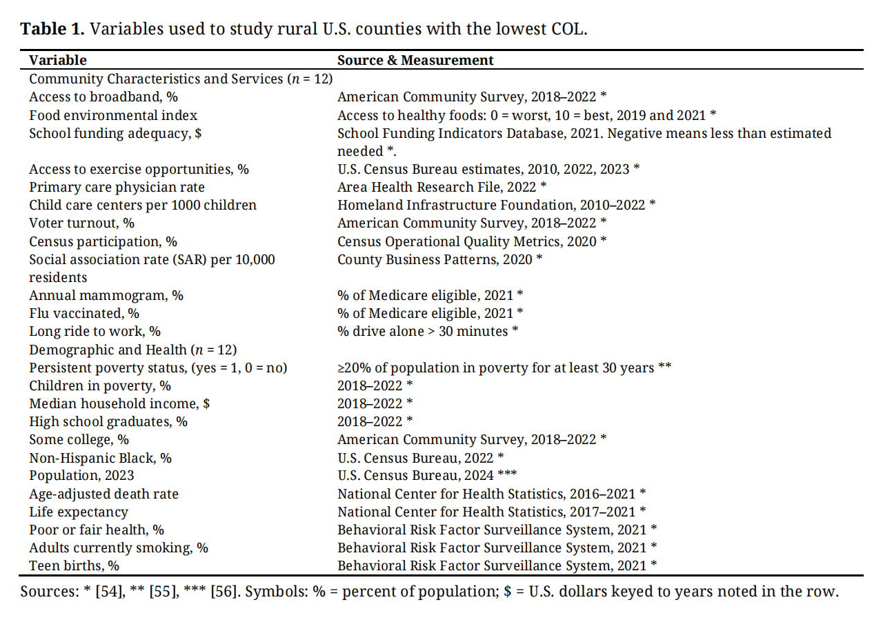Table 1. Variables used to study rural U.S. counties with the lowest COL.

Q1 asked whether the areas with the lowest COL in the United States are disproportionately located in rural areas. We used Niche’s COL grades and rankings for every U.S. county. Rural counties represent 34 percent of U.S. counties. If they are disproportionately found to have the lowest COL ranks, then the proportion should be significantly higher than 34 percent.

Q2 required that we compare services and community assets between the lowest COL rural counties and other rural ones. We selected ten percent of the rural counties with the lowest COL (111 of the 1105 counties) to compare with the remaining ones. T-tests were used to compare the means of the two sets across the 12 community characteristics and service variables listed in Table 1.

To examine the variation among the lowest-COL rural counties in terms of services, demographics, health, and local environmental conditions (Q3), we began by using principal components analysis. Principal components analysis uses matrix algebra to create a new set of uncorrelated multivariate components that capture most of the variance of the original variables. In this case, it made 12 new statistical components from the characteristics and services variables listed in Table 1. The four strongest components were used to assign a score to each county, and these scores were used to classify the 111 lowest-cost rural counties into four service-attribute groups (see below).

The groups with the most (n = 17) and least services (n = 16) among the four sets of counties were compared for evidence of gentrification and cooperation. As the number of cases was small, the results for the counties showing the most evidence of gentrification (n = 7) were further evaluated using a case-study format.

RESULTS

The 100% rural counties represent 34 percent of all U.S. counties. Eighty-six percent of the 100 U.S. counties with the lowest COL were rural, a striking difference.

Table 2 compares the lowest-COL rural counties (n = 111) with approximately ten times as many other rural counties (n = 994) across the twelve dimensions of community characteristics and services. The results are not subtle. Across all 12 variables, the outcomes for the lowest COL counties are less favorable than for the other rural counties, with 11 of the 12 being statistically significant at p < 0.05. (Flu vaccination is the exception.).

TABLE 2

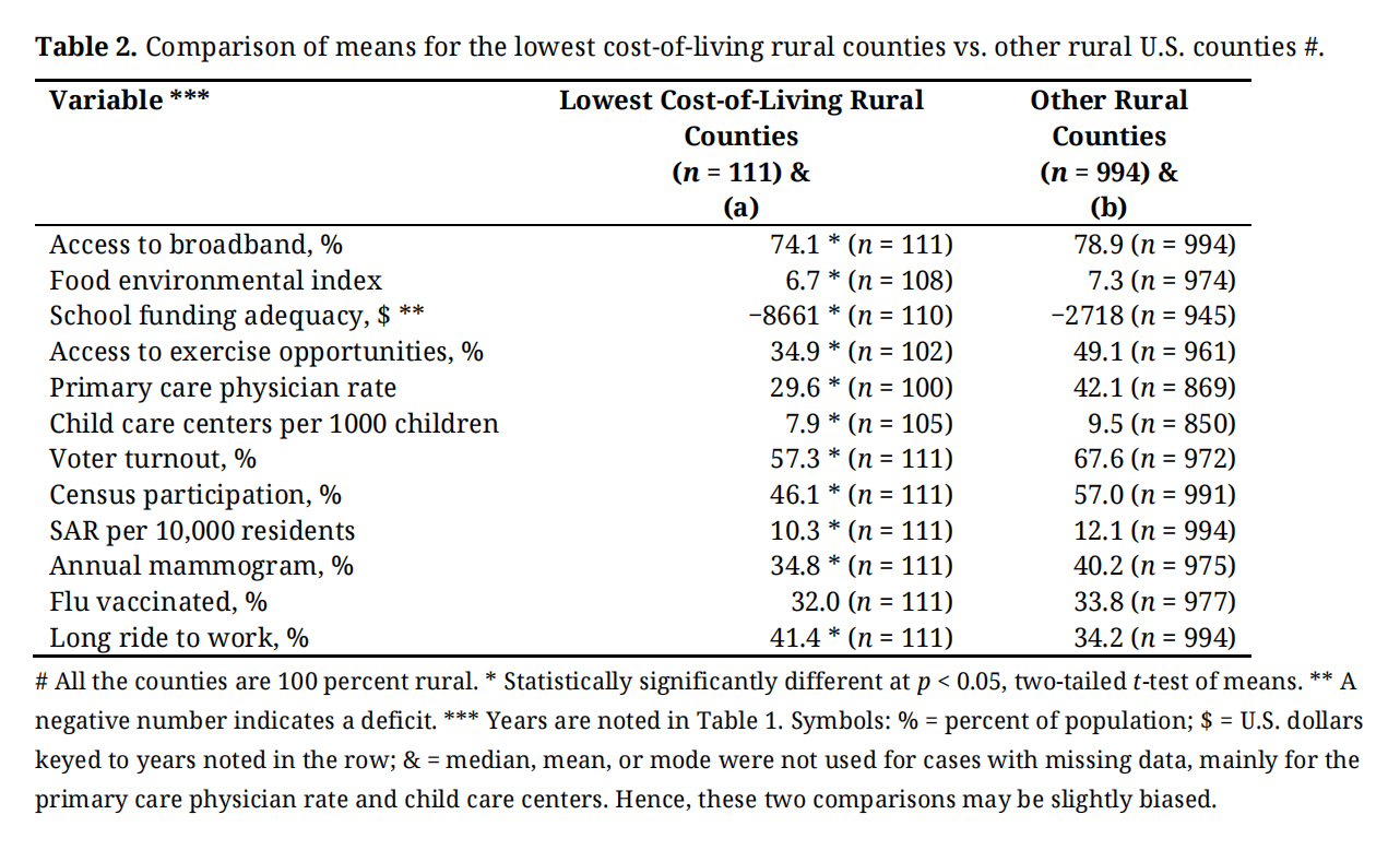Table 2. Comparison of means for the lowest cost-of-living rural counties vs. other rural U.S. counties #.

Of the 111 lowest-COL rural counties, 104 are located in the South, and the other seven are in the Midwest. One cluster is located in Appalachia, comprising West Virginia (n = 16) and Kentucky (n = 16), as well as a small portion of Appalachian Virginia. A second cluster parallels the Gulf Coast, including parts of Louisiana (n = 6), Mississippi (n = 11), Alabama (n = 11), and Georgia (n = 9). A third group is found in Oklahoma (n = 13) and Arkansas (n = 12) (see Figure 1). Readers interested in replicating the Niche data should sign into Niche and query “2025 counties with the lowest cost of living.” Martin County (KY) will be the first listed.

FIGURE 1

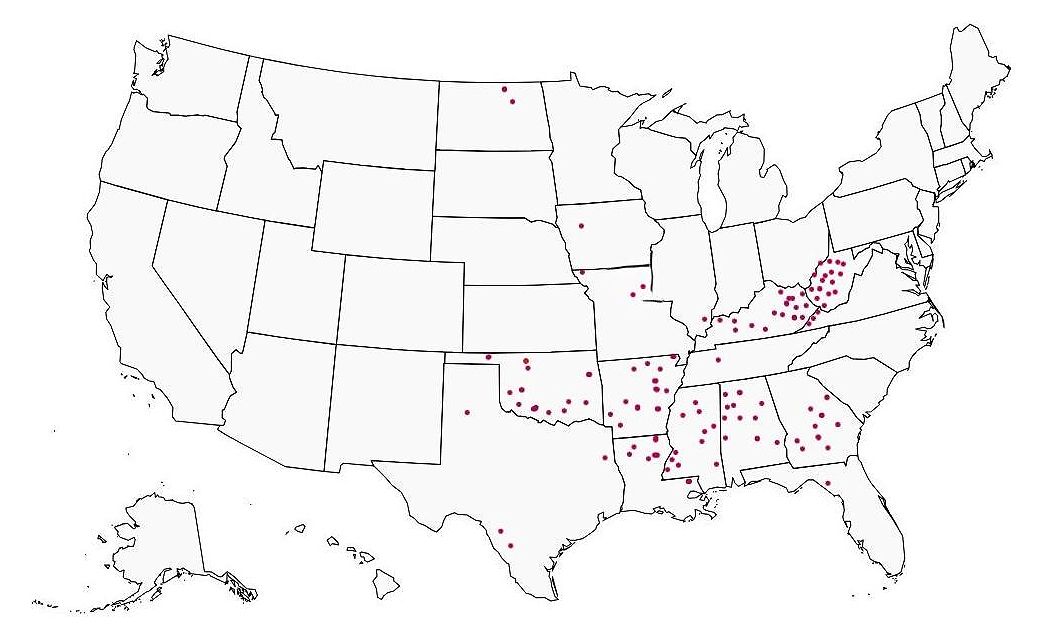Figure 1. Location of 100 percent rural U.S. counties with the lowest cost-of-living, 2024.

The results of the principal components analysis are presented in Table 3. The four components accounted for 62 percent of the variance from the original 12 variables. The correlations with R values greater than 0.40 are listed for the 12 variables. Component 1 identifies places with markers of high personal and group participation. Component 2 shows those with higher local school funding, access to broadband, and a higher food environmental index, but low voter turnout. The third component describes a county’s access to exercise and work. Component 4 points to areas with relatively high numbers of physicians but limited access to exercise opportunities.

TABLE 3

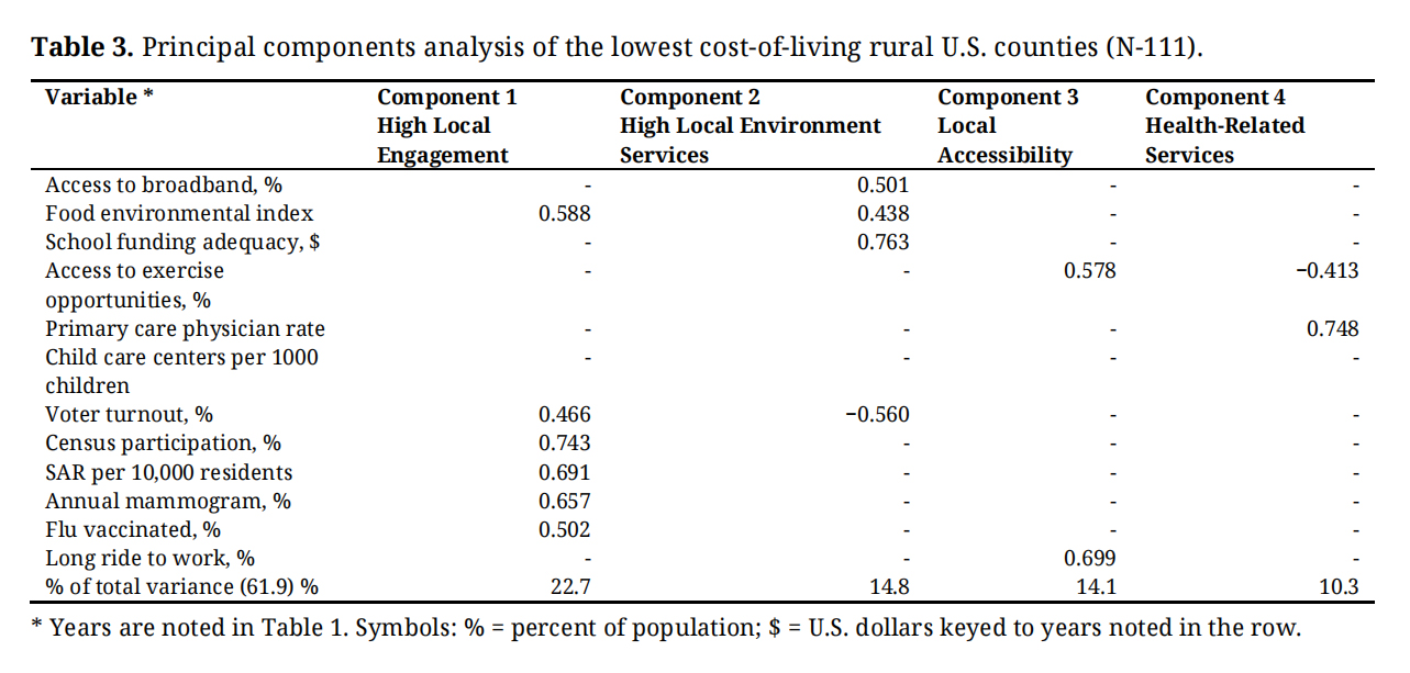Table 3. Principal components analysis of the lowest cost-of-living rural U.S. counties (N-111).

We wanted to compare the extremes of all 111 places, a challenge due to the small number of cases. Thus, we compared places with the best and worst outcomes using standardized scores for each of the 111 rural counties, classified using a transparent and straightforward rule. Seventeen of the counties had positive scores (higher than the average) for all four components. We referred to them as “most services and related attributes.” As Table 4 shows, Oklahoma had eight of the 17 counties. We compared them with 16 counties with the least services and associated attributes (below average for all four measures). Notably, all 16 were classified as persistent poverty counties by the U.S. Census Bureau. The counties with the most and least local services and related attributes are listed in Table 4. Oklahoma represents the high-service group of counties, while Kentucky and West Virginia represent the low-service counties.

TABLE 4

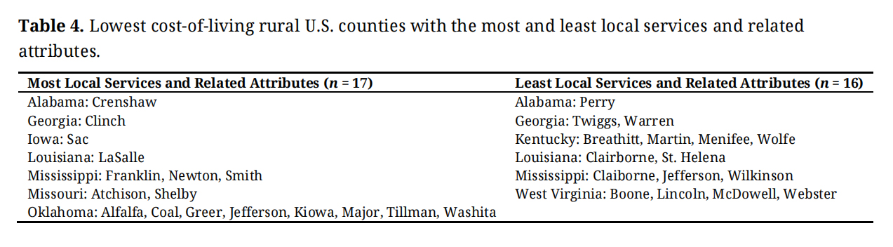Table 4. Lowest cost-of-living rural U.S. counties with the most and least local services and related attributes.

We then compared the two sets using data from the Niche database, which includes public school quality, housing, family environment, jobs, and the overall Niche rating. Counties with at least B−/B (average) or higher ratings were considered positive. Nearly every county was at or above average for each of the five measures. Some were notably above. Niche adds notes to their county profiles. Seven Group 1 profiles note that the county is an excellent place for retirees.

In contrast, the profiles for the 16 Group 4 counties are markedly different. None are noted as good places for retirees. Their median overall rating was C−, and their median rating for local public schools was D.

We examined two additional ideas from the literature. The first is that a local college makes a positive difference in the rating of rural counties. About half of the counties in both groups had at least one two-year local college or technical training center. The second idea we pursued concerns the distance from the center of a rural county to the center of a metropolitan region. Here we saw a difference. Eight of the Group 1 high-service counties were within a one-hour drive to a city center, and the median travel time was 64 minutes. Two of the 16 Group 4 low-service counties were within a one-hour drive, and the median travel time to the city center was 78 minutes.

The final piece of our Q3 analysis was to ground-truth the quantitative data analysis on seven counties with short case studies of counties for evidence that met Nelson’s criteria [41] of having a disproportionately high number of seniors (65+) and Hispanic Americans, as well as evidence of local cooperation within communities. These seven were chosen from the 17 counties in the most service group of counties. Sac, IO; Atchison and Shelby, MO; Alfalfa, Coal, Jefferson, and Major, OK, have higher proportions of both senior residents (65+) and Hispanic Americans, markers of gentrification, as per Nelson et al. The differences between these seven and the other 10 high-service counties, however, were slight. The medians were almost the same. We do not consider these limited case studies sufficient for generalization. They are diverse in many ways, as stated below, but do represent the possibility of a case study approach that could lead to policy-significant insights about why some low COL places can provide more services than many others with low COLs.

Regarding cooperation, we identified local attributes, special conditions, and challenges by examining materials posted by local and state governments, the media, local not-for-profit organizations, and companies located in the seven counties. We found information on local groups attempting to cope with the ongoing threat posed by population decline, particularly among young and talented individuals, the economic uncertainties associated with relying on agriculture or mining, and the increasing pressure on local budgets. In other words, rather than major gentrification, we found evidence of local cooperation in the best service counties.

We note more evidence of local cooperation by the social association ranks of the seven counties (1, 2, 3, 4, 19, 42, and 67) in their respective states, which average 91 counties each. All seven have relatively high flu vaccination rates, voter turnout, and census participation, and most have lower rates of violent and property crime. These empirical data provide additional indirect evidence of civic involvement and local cooperation. Niche rankings for a good place to buy a house (housing), a good place for retirees (retirees), the lowest COL, and the social association rate (SAR) for the seven counties are found in Table 5. Clearly, this number of cases is too small for generalization. However, it is encouraging regarding the role of cooperation through community activity.

TABLE 5

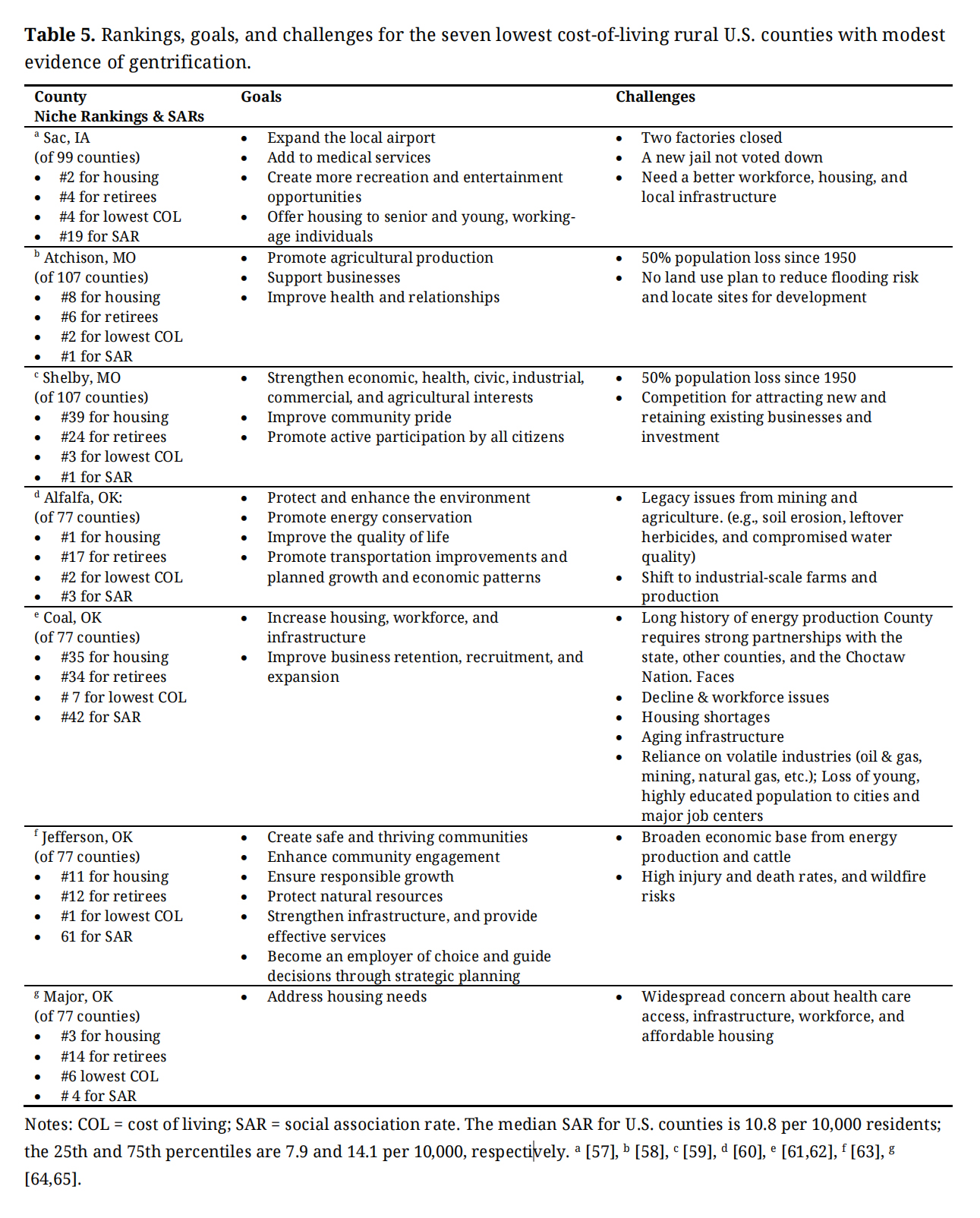Table 5. Rankings, goals, and challenges for the seven lowest cos t-of-living rural U.S. counties with modest evidence of gentrification.

DISCUSSION

We begin by summarizing and answering the three research questions. Question 1 asked whether the lowest-COL areas are disproportionately found in rural areas. We found 86 percent of the one hundred lowest-COL places are in 100% rural counties, primarily in the South and Midwest, and across a band that stretches from Mississippi eastward to Georgia. Results for question 2 showed that the lowest-COL rural counties have fewer community services, lower socioeconomic status, and poorer health outcomes compared to other rural counties. Question 3 probed variations among the 111 lowest-COL rural counties, finding significant differences within the set. At one pole, extremely distressed counties are classified as persistently poor. At the other end of the spectrum are the 17 lowest-COL rural counties, which have more positive indicators for services, socioeconomic status, and job opportunities. Several counties on the latter pole appear to demonstrate modest evidence of gentrification. Still, the case studies reveal limited opportunities due to massive population declines, brain drain, and legacy issues in mining, manufacturing, and agriculture. Even the most successful rural counties face an ongoing challenge in maintaining the cooperation necessary to survive and move forward.

One limitation of this study is the sparse data at a scale smaller than the county level. To address this limitation, we used only counties that are 100 percent rural. Using data on less than 100 percent rural ones could mask significant intra-county variation and yield spurious results. Another limitation is the availability of quality-of-life information for all U.S. counties, particularly regarding noise pollution, air quality, and water quality. Lack of such information poses uncertainty for those seeking to move to rural areas with a lower COL, quieter surroundings, physical attractions, and other rural attributes. Such a move is tempting, especially if telecommuting is possible, and entertainment and educational opportunities are within an hour away. The consequences of substantial growth in rural areas, however, could include the displacement of existing residents who face competition for properties, loss of control over local policies, disruption of local environments, and lead to political disputes with long-term residents. In other words, a more sustainable solution for some may upset others’ sustainable environment.

We end by returning to some of the issues raised in the introduction. We issued a warning to potential migrants about the importance of being diligent before deciding whether to move or stay, as well as where to relocate. We relied heavily on databases that were easily accessible to the public. We used multivariate statistics to classify all the rural counties in the United States and compare them to other U.S. counties. However, once we completed these analyses, we delved into smaller databases that are searchable by potential movers, allowing them to view summaries about specific places and neighborhoods. However, the case study method is replicable by many Americans facing an important choice that will likely influence their future and the future of others, and we strongly advocate for this approach to be used.

Regarding local policy formation, we recognize the bind of economic decline that many rural areas, especially those in this study, face. Individuals interested in relocating to a low-cost rural area should be diligent about their objectives and tolerances for reduced services. In some cases, the gap between urban-suburban and 100 percent rural areas in the United States is pronounced. Local politics must be considered in investigations before a move, as the existing local community may not welcome migrants, viewing them as instruments of change. There may be friction with long-term residents about the local environment and embedded culture. Migrants to these areas need to be prepared to collaborate effectively with local groups to enhance the quality of life in rural communities and increase their chances of a successful transition. Before moving, they must list and discuss their goals to achieve a sustainable environment, use publicly available data, and review local community plans and media information to increase their knowledge. If they take these steps, they may avoid becoming among those who move to a lower COL area that they assumed would be a marked improvement, only to be disappointed and try to return to the place they left.

Local government officials face the challenge of balancing the need to avoid becoming the next ghost town and losing young people to other areas, versus trying to add assets without displacing many of their residents and radically changing the local culture and politics. To support all stakeholder groups, we note that the literature suggests processes that emphasize proactive communication with stakeholders (including residents, businesses, realtors, and investment groups) about their needs, preferences, and perceptions. Sufficient policy-linked literature does not exist. We argue for conducting trustworthy surveys of current residents, recent migrants to rural areas, and local officials to document their perceptions and experiences of urban-to-rural migration in their communities. It is essential to understand their goals, their experiences, and recommendations for improving the experiences for the next potential wave of migrants.

It has taken the United States many decades to gain insight into the experiences of people who have moved from rural areas to urban centers. We are not naive enough to believe that conflicts can be avoided. It is, however, realistic to expect that dispassionate and trustworthy research can identify processes that will enhance the benefits and mitigate the pain for migrants, current residents, and their local governments.

DATA AVAILABILITY

The authors generated no new data. The sources of the data are listed in the text and references. Readers interested in seeing the data should contact the authors.

AUTHOR CONTRIBUTIONS

M.R.G. conceptualized the study, applied the methods, chose the data and software, prepared the initial draft, including the map. D.S. concurred with and expanded the conceptualization, added to and edited the writing, compiled and edited the references. Both authors have read and agreed to the published version of the manuscript.

CONFLICTS OF INTEREST

The authors declare that they have no conflicts of interest.

FUNDING

No funding was received for this research.

ACKNOWLEDGMENTS

We appreciate the helpful comments of the multiple reviewers and editors of this work.