Location: Home >> Detail
J Sustain Res. 2026;8(2):e260045. https://doi.org/10.20900/jsr20260045

Department of Human Resource Management, College of Business Administration, Prince Sattam Bin Abdulaziz University, Al Kharj 11942, Saudi Arabia
Background: Human resource management has undergone a fundamental transformation due to the widespread adoption of digital technologies, prompting organizations to align strategic digital solutions that enhance workforce excellence and global competitiveness. Purpose: This paper examines the relationships between the drivers of digital integration in HRM and workforce transformation and competitiveness, as Saudi Arabia advances its Sustainable Development Goals (SDG) agenda across all sectors in line with Vision 2030. The moderating effect of challenges among those factors is also examined. Methods: A semi-structured survey questionnaire was used to collect research data from industry HR experts. Exploratory factor analysis (EFA) was conducted using Jamovi software to examine the factor structure of the construct, and confirmatory factor analysis (CFA) validated the hypothesized measurement model. Furthermore, the hypothesized relationships among study variables were tested using Jamovi software. Findings: Findings revealed a strong positive relationship between digital integration enablers and workforce transformation, which in turn showed a positive relationship with competitiveness. Conversely, digital integration barriers demonstrated a strong negative moderating effect on the independent variables. Originality/Value: The study’s originality lies in empirically modeling the enablers and inhibitors of digital HRM, offering novel insights for academic scholars and practitioners regarding strategic priorities, as well as for policymakers in identifying institutional and policy gaps critical for sustainable organizational advancement.
SDG, Sustainable Development Goals; EFA, Exploratory factor analysis; CFA, Confirmatory Factor Analysis; KMO, Kaiser-Meyer-Olkin; CR, composite reliability; AVE, Average Variance Extracted; DHRM, Digital Human Resource Management; VIF, Variance Inflation Factor; RBV, Resource-Based View; TAM, Technology Acceptance Model; UTAUT, Unified Theory of Acceptance and Use of Technology; DCT, Dynamic Capabilities Theory; AI, Artificial Intelligence; IoT, Internet of Things; ICT, Information and Communication Technology; NCA, National Cybersecurity Authority; PDPL, Personal Data Protection Law; HRA, Human Resource Analytics; HRIS, Human Resource Information Systems; VR, Virtual Reality
Digital HRM (DHRM) refers to the incorporation of modern digital technologies into human resource management, substituting traditional manual processes with automated, data-driven, and interconnected systems to improve HR functions such as recruitment, development, and retention [1]. Workforce transformation is the strategic alignment of employee roles, skills, and HR practices triggered by technological integration within an organization to remain competitive in a rapidly evolving environment [2]. Competitiveness is the ability of an organization to utilize its internal resources, capabilities, and strategic advantages to maintain or enhance its market position and business performance in a dynamic environment [1]. Although many organizations worldwide have implemented technological changes, the process remains challenging in Saudi Arabia, a nation undergoing profound social, economic, and technological transformation. Under Vision 2030, and within the framework of Sustainable Development Goals (SDGs) 8 and 9, the nation places strongly emphasizes on innovation, sustainability, and workforce development as essential foundations for transformation [3]. In this context, incorporating digital technology into HRM is vital for advancing national competitiveness and transforming the workforce. Research studies have reported that organizations frequently encounter numerous drivers, such as digital literacy, preparedness for emerging challenges, and the development of a skilled workforce [4], as well as barriers related to cyber threats and data privacy [5] and persistent challenges involving regulatory constraints, cultural barriers, digital divide [6], infrastructure limitations, and shortage of skilled talent, and rigorous ethical standards [7]. To ensure the successful implementation of digital HRM and promote workforce transformation, sustainability, and competitiveness, it is imperative to understand these drivers and barriers.
The existing literature has advanced in various aspects of digital technologies in HRM and their significant contributions to strengthening organizational performance and competitiveness. However, several critical gaps remain unaddressed. First, major studies have predominantly investigated digital HRM from the triple bottom line sustainability dimensions [8] in isolation, namely environmental [9], social [10–13], and economic sustainability [14,15] with no integrated framework for sustainable workforce transformation and competitiveness. Many studies have reported that, while digital HRM practices are associated with agility, innovation, and performance, sustainability is commonly addressed implicitly rather than as a central outcome [16–19]. Consequently, this approach limits the extent to which digital HRM capabilities are utilized for sustained workforce transformation and competitive advantage. Secondly, many studies in the context of Saudi Vision 2030 are largely descriptive or fragmented. For instance, prior research has emphasized the impact of digital HRM in reinforcing national reforms, Saudization, and workforce participation, without proposing a theory driven empirical model that connects digital HRM, workforce transformation, and competitiveness within a holistic framework [20–23]. This subsequently raises questions about how digital HRM contributes to sustained competitiveness at the national level. Third, most studies are based on single frameworks, namely the Resource Based View (RBV) or technology adoption models. Furthermore, they lack connections to theoretical perspectives, including the Technology Acceptance Model (TAM/UTAUT), dynamic capabilities theory (DCT), and institutional theory, which are critical for explaining: (i) the rationale for organizations’ adoption of digital HRM, (ii) employee acceptance and utilization of these technologies, and (iii) the extent to which such capabilities are converted into sustainable outcomes [16,24–26]. Fourth, the existing literature has understudied contextual drivers and barriers to digital HRM adoption. Determinative factors such as national policy directives, structural challenges, and organizational motivations are often discussed separately, with partial attention to integrated empirical models explaining workforce transformation [18,25,27].
Therefore, the present study investigates the efficacy of digital integration in HRM for Saudi workforce transformation and its subsequent influence on gaining a competitive advantage. It also examines whether the challenges of DHRM negatively moderate the relationship between enabling factors and workforce transformation. Accordingly, the study develops the following research questions to address its objectives.
(1)
(2)
(3)
Digital transformation has become an integral component of HRM, improving both administrative efficiency and strategic capability through the adoption of modern technologies, such as artificial intelligence, analytics, and digital platforms. In the context of Saudi Arabia’s Vision 2030, which emphasizes digitalization and human capital development, a multi-theoretical perspective is essential to understand how digital HRM contributes to sustainable workforce transformation.
From the viewpoint of RBV theory, sustainable competitive advantage emerges from valuable, rare, inimitable, and well-organized resources [28]. In this context, digital HRM including technological infrastructure, analytics capabilities, and digitally skilled employees constitutes a strategic organizational resource that enhances competitiveness. Extending this perspective, DCT explains how organizations build and sustain advantage by sensing opportunities, seizing them, and reconfiguring resources in response to environmental changes [29]. In HRM, this is reflected into sustained digital systems that support reskilling employees, and redesigning HR processes in response to dynamic technological and organizational demands.
At the employee level, the TAM explains employees’ adoption of digital HR technologies based on perceived usefulness and ease of use Davis (1989) [30]. According to this theory, the success of digital HRM depends on the level of employee acceptance and may be ineffective if employees perceive it as complex. Furthermore, institutional theory, explained by Greenwood and Meyer (2008) [31] addresses the role of external pressures in shaping organizational behavior. In the context of Saudi Arabia, policy directives, cultural change, normative expectations, and national initiatives drive digital HRM adoption, which was also asserted by past studies [32]. However, these pressures may also generate challenges because of insufficient organizational readiness, skills, or infrastructure [32].
Collectively these four theories demonstrate how Saudi Arabian organizations can effectively utilize digital technologies in HRM to strengthen sustainable workforce transformation. From the RBV perspective, organizations must develop unique digital HR capabilities with advanced HRIS platforms, data analytics competencies and HR professionals possessing the latest digital skills. From the DCT perspective, organizations must foster dynamic capabilities to sense emerging HR technology trends, seize innovation opportunities, and continuously reconfigure HR functions to maximize digital value. Further, TAM perspectives offer conceptual insights into investing in user centered design, training employees, clearly communicating the benefits of digital HR tools, and supporting their acceptance and effective utilization [33,34]. Within the framework of Saudi Vision 2030, this study critically examines the key drivers and barriers of DHRM initiatives and empirically analyzes their relationship with workforce transformation and competitiveness. The retrospective literature review presents different views of this strategic digital integration.
Drivers of Strategic Digital Integration in HRMUnder the Vison 2030 initiatives, emerging technologies, such as artificial intelligence (AI), the Internet of Things (IoT), blockchain, and advanced ICT systems are redefining the Saudi economy and society by reducing its dependency on oil, diversifying the economic base through renewable resources, and focusing on sustainable development [35]. AI is a catalyst for innovation, enhancing decision-making and increasing productivity in fields such as healthcare, education, and manufacturing [36]. IoT applications have enhanced sustainability and efficiency in NEOM, agriculture, and Riyadh projects [9,37]. Al-Kahtani et al. (2022) [38]; and Alateeg and Alhammadi (2024) [39] stated that blockchain adoption in the finance sector has improved trust and transparency in e-government and supply chains, ensuring secure transactions.
To explain employees’ and managers’ adoption of digital HR technologies, TAM and UTAUT provide a micro-level behavioral lens. Meta analytic evidence in digital HRM finds that UTAUT type models effectively consolidate prior fragmented work and predict adoption across HR contexts by emphasizing performance expectancy, effort expectancy, social influence, and facilitating conditions [40]. Broader technology adoption reviews argue that TAM and UTAUT remain core frameworks, but they often must extend with context specific factors such as trust, digital skills, organizational support, and culture to explain adoption in complex digital transformation projects [33,34]. These models can ground hypotheses that perceived usefulness and ease of use of HR portals, AI supported HR tools, and HRIS, shaped by training, digital culture, and management support, drive intention to use and continued use among Saudi employees and HR staff, which in turn enables workforce transformation.
These advancements are fundamentally enabling new possibilities for organizations’ sustainable growth, efficiency, and workforce transformation. In this context, digital platforms in e-government applications such as Absher and Tawakkalna have enhanced efficiency and citizen engagement by providing faster and more reliable public services [41]. Alrashdi et al. (2024) [42] studied the impact of digital proficiency on transforming the Saudi healthcare workforce. The study underscored digital competence as a hallmark of the modern healthcare system, highlighting the use of modern technologies such as AI in telemedicine, electronic health record management, and the streamlining of daily operations for more efficient workflows. The automation of administrative processes has improved efficiency, allowing practitioners to focus on personalized care, and ultimately leading to greater patient satisfaction. However, the study also highlighted persistent skill gaps, outdated training models, resistance to change, and inequitable access to infrastructure as critical challenges in achieving successful digital proficiency. Furthermore, intensive mentorship and the promotion of digital education are recommended as vital strategies to overcome such obstacles [43].
Vision 2030 has introduced a strong institutional and policy framework to promote technological adoption and economic diversification. Al-Ayed (2022) [44] and Saeed et al. (2023) [45] asserted that these technologies are enabling industrial advancement, smart city development, and the establishment of a secure governance system. Projects such as the National Strategy for Data and AI (NSDAI) are part of Saudi Arabia’s vision to become a global center for AI by 2030 [7]. Alrubaidi (2024) [41] argued that government led projects, such as e-governance platforms for Saudi citizens and residents, are essential for efficient and secure transactions, with improved trust, transparency, and accountability. The Abir project, a digital currency launched by the Central Bank of Saudi Arabia in cooperation with the Central Bank of the UAE, demonstrates that the Kingdom maintains a secured digital infrastructure and supports financial innovation [38]. Blockchain has improved transparency, trust, and efficiency in financial services logistics, and government processes. Furthermore, ICT has increasingly contributed to economic diversification, for instance, through e-government and digital inclusion.
Many studies support digital initiatives that contribute to the efficient, competitive, and sustainable growth of the nation. Likewise, the operation of systems has been transformed by IoT to facilitate real-time data flow and processing, especially in smart cities such as NEOM, with the integration of intelligent energy systems and automated infrastructure [9,37]. Therefore, these enablers are categorized as technological, organizational, institutional, policy, sustainability, and performance drivers.
Digital HRM and SustainabilityTraditional HRM primarily focused on administrative efficiency, whereas DHRM, also known as e-HRM, represents a strategic technological innovation aligned with human-centered practices [3]. It improves efficiency, accuracy, transparency, and decision-making by incorporating advanced digital technologies such as human resource analytics (HRA) and automation in HR processes [46,47]. For long-term organizational adaptability, these practices promote sustainability in workforce management through socio-cultural (inclusion, well-being, and diversity), economic (operational efficiency), and environmental (reduction of ecological footprints) dimensions of workforce management [48,49]. Through DHRM, many repetitive HR tasks have been automated via documentation systems, cloud-based platforms, and virtual onboarding, leading to paperless processes [50]. Because AI technology is predictive in nature, it facilitates factual and evidence-based HR decisions, forecasts workforce needs, ensures justified performance appraisals, and enables personalized employee engagement strategies that improve retention and reduce turnover rates [51]. Furthermore, it enhances organizational agility and adaptability by managing human capital in support of global sustainability [52], thereby integrating technological innovation with sustainable development in alignment with Vision 2030 goals [3,47]. In relation to RBV and DCT perspectives, studies provide a strong theoretical foundation suggesting the digital HRM systems and HR professionals’ digital skills constitute valuable, rare, inimitable, and non-substitutable resources that underpin competitive advantage [53–57]. DCT explains how Saudi organizations sense, seize, and reconfigure these digital and human resources to respond to rapid technological and labor market change. Studies show that integrating digital technologies and individual capabilities into organizational innovation capability is central to HRM digital transformation and to sustaining performance in turbulent contexts [58,59]. Empirical work on digital HRM and AI augmented HRM, demonstrates that HR analytics, AI in recruitment and retention, and information system ambidexterity act as dynamic capabilities that enhance productivity, agility and sustainable performance in emerging economy settings [54,56,57,59]. This directly supports hypotheses linking digital HRM practices in Saudi Arabia to sustainable workforce transformation and competitiveness. Therefore, the following hypothesis is proposed:
Hypothesis (H1). Digital HRM drivers will have a significant positive influence on workforce transformation.
Sustainable Workforce Transformation and CompetitivenessDHRM primarily acts as a mediating mechanism between technology adoption and corporate performance, as it promotes competitiveness by transforming the workforce into a more flexible and capable one. It has effectively reshaped the workforce to meet the adaptation requirements of industry 4.0, through targeted upskilling and reskilling initiatives, closing skill gaps and enhancing the overall quality of human capital [60,61]. HR interventions equip employees with digital skills and digital literacy, demonstrating significant improvements in adaptability and innovation. Furthermore, Ruiz (2024) [62] noted that modern technologies digitize routine tasks, support data-driven decision-making, coordinate cross-functional activities, and enable rapid responses to dynamic market changes. Concurrently, DHRM has significantly shifted HR roles and digital culture, moving from administrative to strategic capabilities and motivating the workforce toward continuous learning, experimentation, and psychological safety [63,64]. N’Dri and Su (2024) [65] highlighted that organizational readiness, and external pressure moderate the conversion of DHRM investments into workforce transformation and, ultimately, competitiveness. Li (2024) [61] and Ruiz (2024) [62] further emphasized that a digitally adaptive culture serves as a pivotal bridge in modern digital strategy. Institutional theory connects these internal processes to the Saudi macro environment. Institutional analyses of Industry 4.0 and digital supply chains show that coercive pressures from regulators and powerful stakeholders significantly shape firms’ digital adoption strategies [32]. In Saudi Arabia, Vision 2030, Saudization policies, and national strategies for digital government and human capital development operate as coercive and normative pressures that push organizations to adopt digital HRM, invest in local skills, and increase women’s participation in the workforce [20]. Digital HRM becomes not only a source of efficiency, but also a legitimacy enhancing response to national transformation agendas, where organizations that align HR technologies and practices with Vision 2030 expectations gain access to resources, partnerships, and reputational benefits [20,32]. In combination, DCT/RBV explain how firms transform digital and human resources into competitive advantage; TAM/UTAUT explain micro-level technology acceptance that enables HR digitalization to function in practice; and institutional theory explains why and how Saudi organizations come under pressure to digitize HR for sustainable workforce transformation. Therefore, it is hypothesized that:
Hypothesis (H2). Sustainable workforce transformation has a significant positive effect on competitiveness.
Challenges of Digital HRM Integration as a Negative Moderating FactorDespite substantial digital progress, Saudi Arabia is encountering technological and infrastructure challenges, with the digital divide as the primary barrier between rural and urban regions in terms of equitable access to digital resources [66]. Furthermore, blockchain and IoT systems are facing integration challenges arising from interoperability and scalability issues [39]. Even today, most sectors are constrained by skill shortages in AI, IoT and cybersecurity, further limiting the effective implementation of digital initiatives [67]. Moreover, cybersecurity and data privacy issues have become growing concerns. Most organizations that rely on digital systems have been exposed to cyber threats, data breaches, and privacy violations [68]. According to Al-Kahtani et al. (2022) [38], most traditional sectors face obstacles such as reluctance to change and organizational inertia, largely because of limited awareness of the long-term benefits of digital tools, which further leads to slow integration and underutilization of digital resources. Al-Motrif (2024) [69] and Alghamdi (2022) [70] also noted a shortage of digital talent and limited women participation in technology related jobs, worsening workforce imbalances and indicating a greater need for investment in digital literacy. Al Fryan et al. (2025) [71] explored how Virtual Reality (VR) serves as an emerging transformative tool for leadership development, digital communication, workplace adaptability, and experiential learning by promoting immersive technologies.
Tripathi and Singh (2024) [72] argued that, due to rapid technological change, many frameworks fail to keep pace necessitating ethically sound frameworks and standards for data protection. Furthermore, high implementation costs, infrastructure limitations, uncertainty in regulatory policies concerning blockchain, and data governance remain significant barriers [39]. Although Saudi Arabia has established the National Cybersecurity Authority (NCA) and enacted the Personal Data Protection Law (PDPL) to reinforce digital trust, consistent adaptation is required to address emerging risks. High implementation costs and unclear regulatory policies regarding data handling and digital standards have also restricted smooth transformation across sectors. At present, there is a significant gap in cybersecurity awareness among the public, which increases susceptibility to social engineering attacks [73]. However, several challenges remain unaddressed concerning usability, contextual relevance and the translation of virtual experience into practical workplace outcomes. Despite these limitations, the study emphasized that VR based leadership training indicates a scalable, innovative, and culturally adaptable approach to empowering Saudi women leaders in alignment with Vision 2030. Hence, digital inclusion, gender equity and cultural acceptance are essential for achieving successful workforce transformation. Despite substantial digital drivers and national initiatives toward Vision 2030, workforce transformation does not occur automatically but depends on the extent of existing barriers. The highlighted barriers related to organizational development, technology acceptance, regulatory constraints, socio-cultural factors, infrastructure gaps, skill shortages, and policy uncertainty can weaken the effectiveness of these drivers. Therefore, barriers moderate the association by either constraining or enhancing the effectiveness of digital drivers in transforming the workforce. From the above conceptual discussion, the following hypothesis is proposed:
Hypothesis (H3). Digital HRM barriers negatively moderate the relationship between digital HRM drivers and workforce transformation.
Although significant growth is evident in digital transformation, past studies have rarely examined how digital HRM opportunities and challenges together stimulate sustainable workforce transformation and competitiveness within the framework of Saudi Arabia’s Vision 2030. Existing research remains fragmented and lack empirical validation of these interrelationships. The proposed conceptual model is presented in Figure 1.
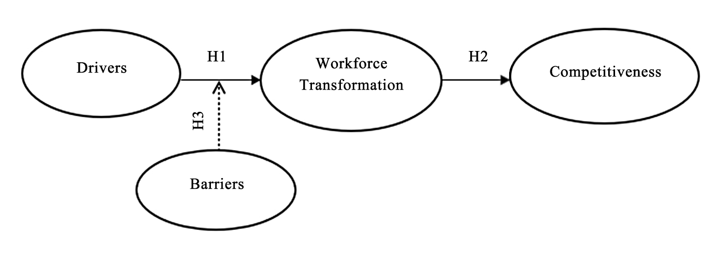 Figure 1. Proposed Conceptual Model.
The study used a mixed-methods design combining expert consensus with primary data from employees across various organizations in Saudi Arabia. This approach provides a holistic understanding of the effects of digital transformation on work processes, skill gaps, and organizational outcomes. Accordingly, the study was conducted in two phases. First, content validity was assessed by evaluating experts’ ratings of the identified constructs and items to develop a strong measurement scale. Second, primary data were collected using a structured questionnaire to conduct empirical analyses and examine the relationships among the constructs.
Construct and Measurement Item development Based on Theoretical FoundationsThe area of study, digital HRM as an enabler of workforce transformation and competitiveness is relatively underexplored. Moreover, the interplay among its key constructs such as drivers and barriers, workforce transformation, and competitiveness, has received limited empirical attention. Extant literature provides conceptual insights; however, existing measurement instruments have not been fully tailored to the Saudi context.
To address this gap, the researcher identified digital HRM drivers and barriers, workforce transformation, and competitiveness as key constructs relevant to the study’s objectives. After extensive content analysis of the literature, key conceptual dimensions were identified to guide item development for each construct. These dimensions were used only as a theoretical basis for generating measurement items (survey statements), rather than being empirically tested as separate factors. For example, the Digital HRM Drivers construct was conceptualized through five dimensions: Vision 2030 alignment, strategic alignment, talent competitiveness, leadership commitment, and technological advancement. Based on these conceptual foundations, measurement items (survey statements) were developed to operationalize each construct [46,47,63]. All measurement items were compiled into a structured questionnaire and evaluated by experts for content validity. Following the CVI assessment, only the most relevant items were retained for the final analysis. Under the “Drivers” construct, previous studies emphasized policy integration, leadership engagement, technological adaptability, and human capital strategies [38]. Accordingly, the final measurement items reflected these underlying themes, including Vision 2030 alignment and national policy, strategic business alignment and efficiency, competitive talent acquisition and retention, leadership commitment and organizational readiness, and technological advancement and global benchmarking. The “Barriers” construct captured challenges identified in prior literature, such as digital infrastructure limitations, organizational inertia, digital competency gaps, and compliance issues related to data integrity and security [74]. These were operationalized into five measurement items: Skill Gaps and Digital Literacy Deficiency, Cultural and Organizational Resistance, Infrastructure and Technological Constraints, Policy, Privacy, and Data Governance Issues, and Cost and Resource Constraints. Workforce transformation highlighted a shift toward a learning culture, organizational agility, workforce empowerment and a framework of digital HRM transformation [60–62]. Accordingly, this construct was measured using items reflecting: Skill Enhancement and Continuous Learning, Flexible and Hybrid Work Structures, Empowerment and Employee Engagement, and Redefining Roles and HR Function. Finally, competitiveness was conceptualized in terms of digital advancement, workforce adaptability, innovative capability, and global positioning [64,65] and is operationalized through items capturing global benchmarking and market positioning, innovation and agility, talent competitiveness and retention, organizational performance and productivity, and strategic global readiness.
To establish content validity, all potential measurement items were compiled into a structured questionnaire and sent to ten HR professional experts currently involved in digital HRM implementation. The experts evaluated each item for relevance and appropriateness using a five-point Likert scale (1 = strongly disagree, 5 = strongly agree). Based on the content validity index (CVI), only items with acceptable values (greater than 0.78) were retained for the final instrument, in line with Lynn (1986) [75]. Subsequently, the validated items were used to develop the final survey questionnaire, which was also measured on a five-point Likert scale. This approach was theoretically grounded and methodologically robust, as expert judgment is widely accepted for establishing content validity in scale development studies. Although multiple conceptual dimensions informed item generation, all constructs were operationalized as unidimensional reflective constructs measured using multiple validated items.
Data Collection and Sampling MethodThe final structured survey questionnaire was distributed online via Google Forms to 600 potential HR employees at operational, tactical, and strategic levels across various firms and sectors in the Riyadh region. The study employed purposive sampling. Although participation was voluntary, informed consent was obtained prior to data collection, with a clear explanation of the research purpose. Data were collected over a two-month period with the help of officials from the information technology and HR departments, resulting in 415 usable responses. The anonymity of respondents was maintained, and the authors declared no conflict of interest. The details of the constructs and measurement items are as follows. “Drivers” is measured with five items. An example statement is “My organizational HR strategies are effectively aligned with Saudi Vision 2030 and national policy goals.” “Barriers” is measured with five items, and an example statement is “Limited digital literacy and a shortage of technical skills among employees impede the effective integration of digital tools in HR functions.” “Workforce transformation” is measured with five items, for instance “I believe sustained skill development and ongoing learning opportunities are necessary for adapting to workforce transformation.” Competitiveness is also measured with five items, such as, “I believe our organization’s benchmarking against global standards improves its market position.”
The study received 415 responses and checked the data for normality, multicollinearity, outliers, and missing data, and it used Jamovi software version 2.7.12 for data analysis. Table 1 presents the demographic characteristics of the participants. The majority of participants were male, aged 31 to 40 years, most held a master’s degree, and had 6 to 10 years of job experience occupying operational-level positions. Most of the organizations were medium-sized enterprises.
Prior to data analysis, several preliminary screening and diagnostic tests were conducted to ensure the adequacy and reliability of the data. Data screening was performed using Jamovi software. Missing data were examined through descriptive statistics, and no missing data were found, meeting the acceptable threshold (<5%) [76]. Outliers were assessed using boxplots and standardized z-scores. As suggested by Rousseeuw & Hubert, 2017 [77], no extreme values exceeding ±3.29 were identified. Skewness and kurtosis statistics were used to assess normality, supported by visual inspection of bell-shaped histograms and diagonal patterns in Q-Q plots. As recommended by Korkmaz et al. (2014) [78], the results indicated that all variables satisfied the normal distribution.
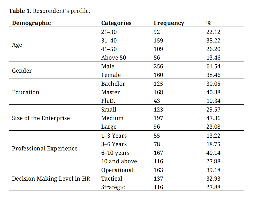 Table 1. Respondent’s profile.
Further, data collection from a single source may introduce potential bias, leading to validity concerns in the study. Therefore, common method bias (CMB) was first tested using Harman’s single-factor test [79] to assess any possible bias issues. All measurement items of the proposed model were grouped into four constructs and examined for the percentage of total variance explained. The single factor explained 26.9% of the total variance, which is below the recommended threshold of 50%, indicating no potential common method bias. Second, variance inflation factor (VIF) and tolerance values, commonly used measures for detecting multicollinearity, were examined to identify any potential collinearity concerns [80,81]. The results demonstrated that the VIF value (3.81) was below the recommended threshold of 5, while the tolerance value (0.262) exceeded the acceptable limit of 0.10 [82]. Therefore, the results confirm that multicollinearity is not a concern in the model.
Exploratory Factor Analysis (EFA)The EFA was conducted using Jamovi software with principal axis factoring and oblimin rotation. The Kaiser-Meyer-Olkin (KMO) measure of sampling adequacy was 0.852, and Bartlett’s test of sphericity was significant at p < 0.001, indicating that the data were suitable for factor analysis. Four factors emerged with eigenvalues greater than 1, as shown in the Figure 2, explaining 92.15% of the total variance. All items loaded above 0.50 on their respective constructs, as presented in Table 2.
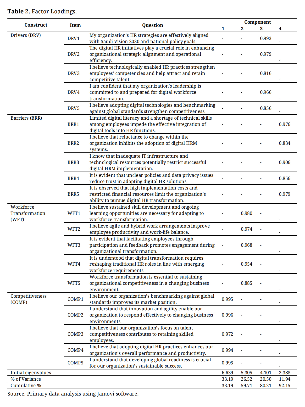 Table 2. Factor Loadings.
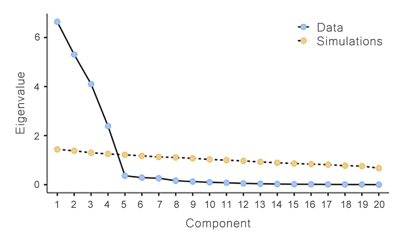 Figure 2. Screen Plot.
The CFA was performed with Jamovi software to test the measurement model. As suggested by Nunnally (1978) [83], construct reliability, indicated by composite reliability (CR) values ranging from 0.961 to 0.996, exceeded the threshold of 0.70. The average variance extracted (AVE), which represents the proportion of variance captured by a construct relative to measurement error, ranged from 0.832 to 0.907, surpassing the 0.50 cutoff suggested by Fornell and Larcker (1981) [84]; and Hair et al. (2020) [82], as shown in Table 3.
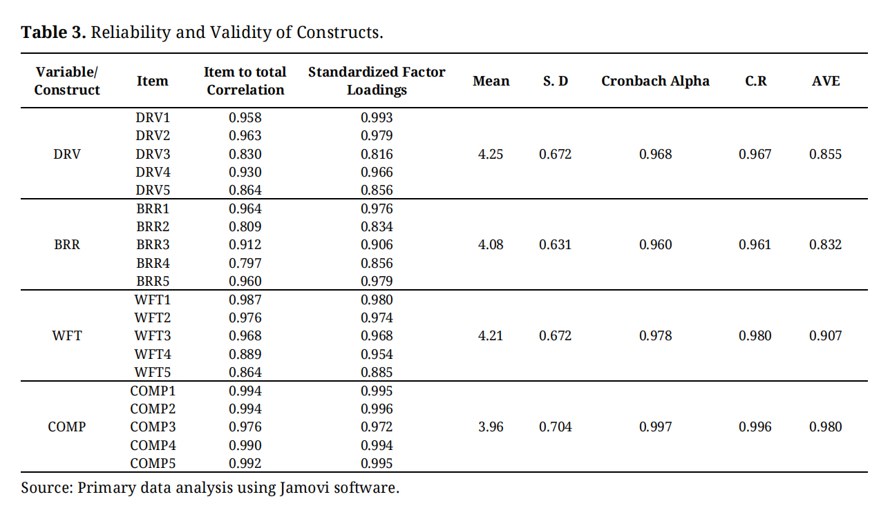 Table 3. Reliability and Validity of Constructs.
Table 4 illustrates the discriminant validity of each factor through the Fornell-Larcker criteria. Table 2 demonstrates that the factor loadings of each item are higher than 0.70 within the range of outer loadings from 0.816 to 0.996. The square root of the AVE for each factor is higher than the corresponding correlation with other factors, indicating clear differentiation from the other constructs. Hence, convergent and discriminant validities are established [84].
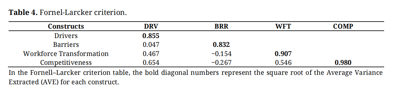 Table 4. Fornel-Larcker criterion.
The fit indices describe how well the model fits the observed data, evaluating both the measurement model and the structural model. Sarkar et al. (2021) [85]; Cheung et al. (2024) [86]; and Khan (2025) [87] highlighted the chi-square test (χ2), comparative fit index (CFI). Tucker-Lewis’s index (TLI), normed fit index (NFI), relative fit index (RFI), standardized root-mean square residual (SRMR) and root mean square error of approximation (RMSEA) as key indicators of model fit. These standard indices guide researchers in addressing model fit issues and drawing reliable conclusions. The measurement model’s metrics are presented in Table 5 while structural model metrics are shown in Table 6. The measurement model demonstrated a good fit, χ2/df (1.875) is within the stipulated range, less than [88], RMSEA (0.044) is also within the limit of 0.06 [89], and SRMR (0.052) is within the range of 0.08 [90]. Also, other model fit indices, CFI (0.943) and TLI (0.934), are within the recommended limits [91,92] and the structural model χ2/df (1.653), RMSEA (0.042), SRMR (0.052), CFI (0.943), TLI (0.932), NFI (0.935) and RFI (0.924) [93] are within the statistically recommended threshold limit referred to Table 6. Covariances between the error terms of selected items within the same construct were added based on modification indices because of conceptual and wording similarity, without affecting the structural paths. These goodness-of-fit indices indicate an excellent fit and confirm the adequacy criteria for further testing the research hypotheses through a structural model.
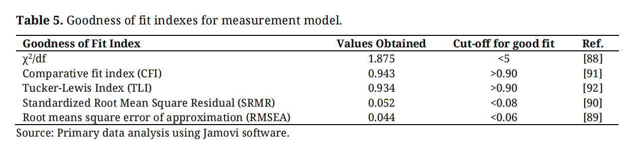 Table 5. Goodness of fit indexes for measurement model.
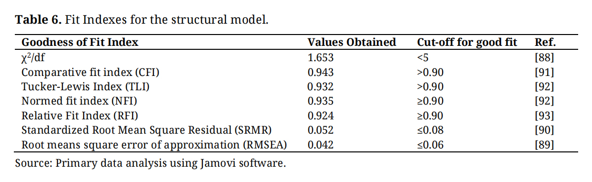 Table 6. Fit Indexes for the structural model.
The path coefficients determined the significance of the hypotheses (CR = critical ratio, β = standardized coefficient, and p-value) as shown in Table 7. A moderately strong and significantly positive relationship exists between DRV and WFT (β = 0.502; CR = 5.976; p < 0.001) and an even stronger and highly significant positive relationship exists between WFT and COMP (β = 0.631; CR = 9.859; p < 0.001), supporting hypotheses H1 and H2. Further, Table 8 presents a significant negative moderating effect of BRR between DRV and WFT (β = −0.216; CR = −2.918; p < 0.014). Figure 3, presents the simple slopes plot of the interaction, showing a strong positive influence of DRV on WFT at low levels of BRR and vice versa, thereby supporting hypothesis H3.
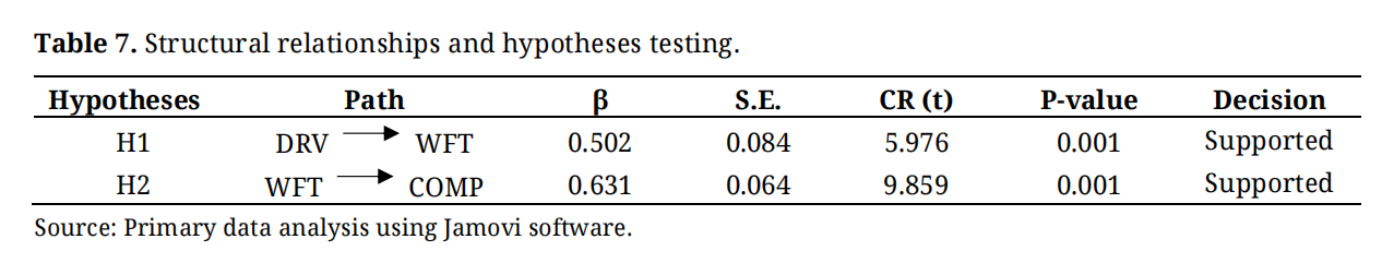 Table 7. Structural relationships and hypotheses testing.
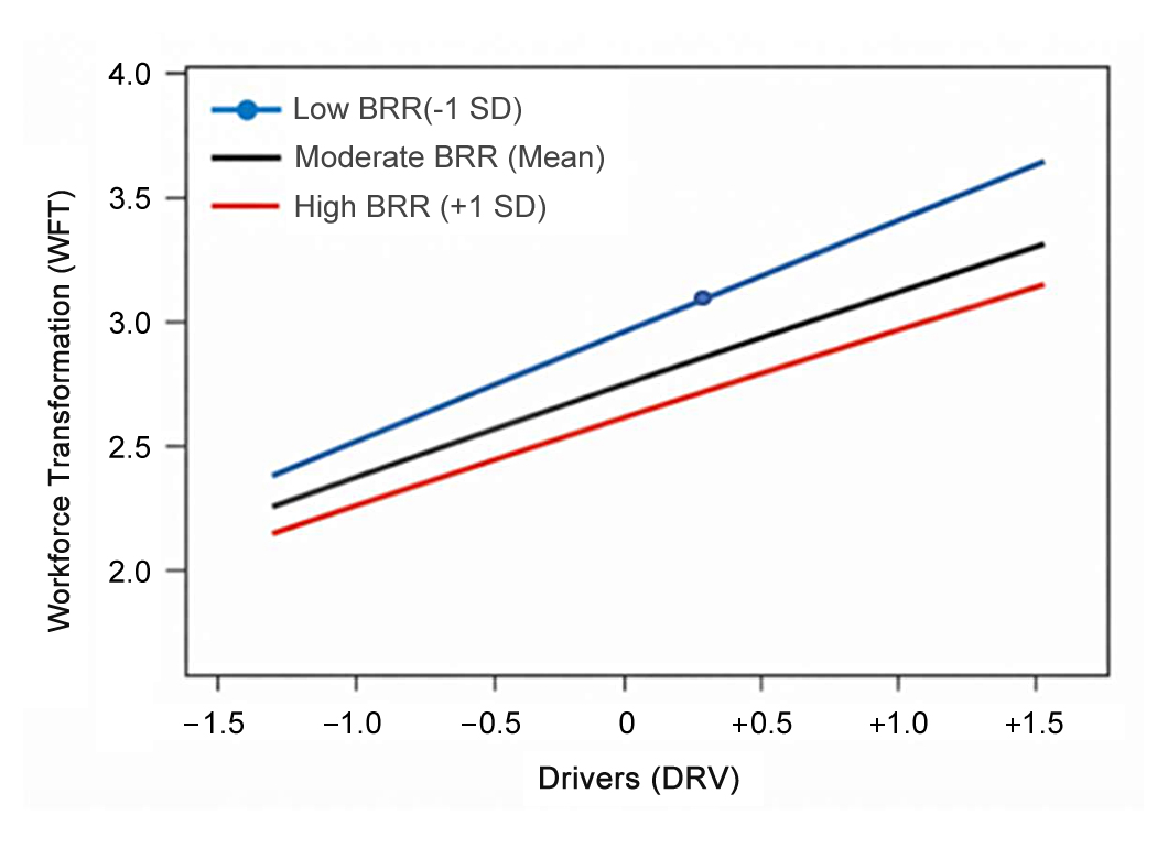 Figure 3. Simple slopes plot of the significant interaction between drivers and workforce transformation in relation to barriers.
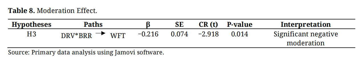 Table 8. Moderation Effect.
The study strengthens the existing literature on Saudi workforce transformation and employee competitiveness by providing empirical evidence on the role of digital HRM. The findings indicate that the drivers of digital integration in HRM promote human capital advancement and competitive readiness. This finding is explained by RBV theory, which postulates that digital HRM systems and employee digital competencies are strategic and inimitable resources that support competitive advantage. Furthermore, from a DCT perspective, firms utilize these digital resources by continuously restructuring workforce skills and aligning them with emerging technological requirements.
Workforce transformation stems from various opportunities, including strategic alignment with Vision 2030, national strategic goals, improved operational performance, and the adoption of digital HR practices. These findings reflect institutional theory, in which Vision 2030 and associated national initiatives act as regulatory and normative pressures that encourage organizations to adopt digital HRM practices not only to improve operational efficiency but also to secure legitimacy within the national transformation program. However, despite these opportunities, prevailing challenges in digital integration have a negative association with workforce development and competitive advantage. From a DCT viewpoint, such constraints hinder organizations’ ability to reconfigure resources strategically, thereby slowing the transformation process. These findings are consistent with previous studies, which emphasize that despite the nation’s visionary mega projects, such as Red Sea Global and NEOM, barriers to technologically skilled and future-ready human capital remain unchanged. They also correspond to the findings of [43], which argued that despite professional initiatives, the nationalization of the labour market, and the early adoption of digital solutions, the workforce still struggles to demonstrate a consistent level of digital capabilities, and relies heavily on foreign expertise in specialized areas. This shows a gap in resource availability and capability deployment as explained by RBV and dynamic capability theories, suggesting that resources alone are insufficient unless they are effectively integrated and reconfigured within organizational processes.
Nevertheless, this study reports that continuous skill development and learning processes engage employees in organizational transformation, which is supported by TAM/UTAUT, which posits that employees’ acceptance and use of digital HR technologies are stimulated by ease of use, perceived usefulness, training and management support thereby reinforcing workforce transformation. Digitally transforming traditional HR operations addresses evolving workforce requirements and strategically enhances competitive capabilities. From the DCT perspective, it is essential to operationalize digital HRM to ensure alignment with the technological ambitions of Vision 2030.
The negative moderating effect of barriers between digital integration, human capital advancement, and competitive readiness is also consistent with previous studies [66,68,69], particularly in the context of reliance on foreign workforce expertise [42]. This finding strengthens the DCT argument that structural and institutional constraints weaken the effective deployment of resources, thereby limiting competitive outcomes. Moreover, these challenges can also be interpreted through institutional theory, in which inconsistency between statutory requirements and organizational capabilities creates a lack of coherence in the transformation process.
The core values highlighted in this study align closely with SDG 8, promoting sustained, inclusive, and productive economic growth through workforce development. Enhanced digital skills, competencies, and adaptability contribute to decent employment opportunities and improved workforce preparedness. From the RBV perspective, these competencies represent strategic assets that support long-term competitiveness, while DCT explains how organizations continuously upgrade these competencies in response to global market changes.
This study provides valuable implications for academic researchers and organizations. From a strategic perspective, it practically illustrates how organizations can systematically develop future-ready employees, improve innovative capacity, reinforce innovation, and enhance strategic adaptability, which are imperative for policymakers and business leaders seeking to reduce dependency on external expertise, promote Saudization, and foster a culture of continuous learning and talent competitiveness. Beyond these practical implications, it theoretically contributes to national economic priorities that promote long-term productivity, competitiveness, and inclusive growth, directly supporting Vision 2030 and SDG 8 goals. Furthermore, the study offers strategic insights for other emerging economies seeking to integrate HRM practices with technological innovation, thereby improving its contextual relevance and global applicability.
This study highlights several limitations. First, the study adopted purposive sampling from organizations located in the Riyadh region of Saudi Arabia, which introduces regional bias and limits the generalizability of the findings to organizations in other regions within the Kingdom. Future studies may consider adopting a probability sampling technique across multiple regions, which can provide more generalizable results. Second, the data were collected at a single point in time using a cross-sectional design, which limits causal inference. Therefore, longitudinal studies are suggested to better understand the dynamic nature of digital HRM adoption and workforce transformation over time. Finally, as this study emphasized digital HRM transformation specifically from an organizational perspective, future researchers may investigate institutional and contextual factors to further strengthen insights into workforce transformation processes.
The study provides strong empirical evidence on the essential role of digital HRM in enabling workforce transformation and enhancing competitiveness within organizations in Saudi Arabia. The study extends digital HRM research by explicitly situating workforce transformation within a sustainability and competitive advantage framework. This study complements previous studies, which have treated sustainability implicitly or focused mainly on operational efficiency outcomes. To ensure methodological consistency and contextual relevance, the study used a mixed-methods approach by integrating expert validation with an online survey instrument. In light of the emerging nature of digital HRM, the study aligns with Saudi Vision 2030 and highlights a critical gap in the literature concerning the drivers, barriers, workforce transformation, and competitiveness from a sustainability perspective. The findings confirm that digital HRM drivers are strategically aligned with Vision 2030 and technological advancement, significantly contributing to workforce transformation, which subsequently enhances employee competitiveness. This highlights the reinforcing role of human capital development in achieving sustainable competitive outcomes, reflecting both social and human capital sustainability dimensions. Furthermore, the study identified skill gaps, infrastructural limitations, organizational resistance, and heavy reliance on foreign labor as persistent barriers to digital integration, reinforcing the negative moderation effect. These challenges underscore potential risks to sustainable workforce development and highlight a strong need for systematic and inclusive digital HRM strategies that support sustainability objectives over time.
In conclusion, the study bridges the gap between Saudi Arabia’s ambitious technological transformation agenda and the practical realities of workforce readiness. It demonstrates that utilizing digital technologies in HRM, such as AI-enabled HR functions, continuous learning platforms, and data-driven decision-making, can accelerate skill development, enhance workforce capabilities, and strengthen adaptability. This research contributes both theoretically and practically, establishing an analytical link between digital HRM, workforce transformation, and competitiveness within a sustainability framework. It provides strategic guidance for organizations and policymakers to prepare a future-ready, human-centered, and nationally empowered workforce aligned with Vision 2030 and supporting the broader goals of sustainable economic growth under SDG 8.
Data will be provided by the author upon reasonable request.
The author declares no conflicts of interest
The authors extend their appreciation to Prince Sattam Bin Abdulaziz University for funding this research work through the project number (PSAU/2025/02/37020).
1.

Copyright © Hapres Co., Ltd. Privacy Policy | Terms and Conditions


